Figure 1: Opening Screen of FreeFem++ CS.
Example 1
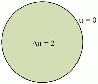
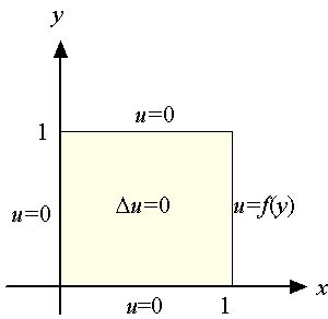
Figure 2: Poisson Equation.
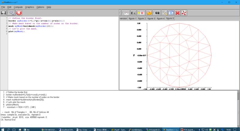
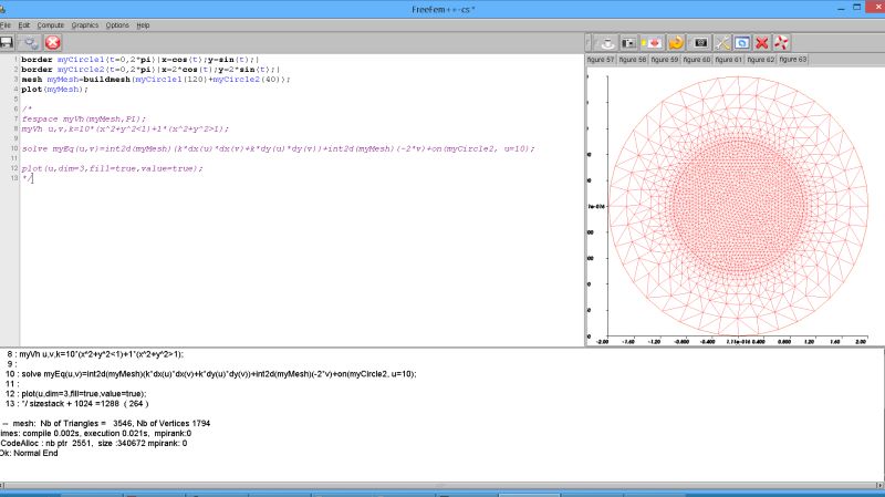
Figure 3: Mesh Generation.
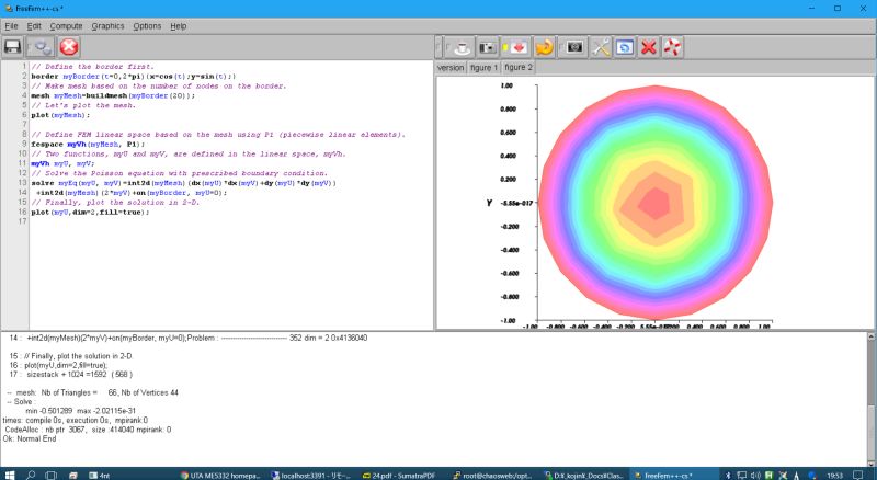
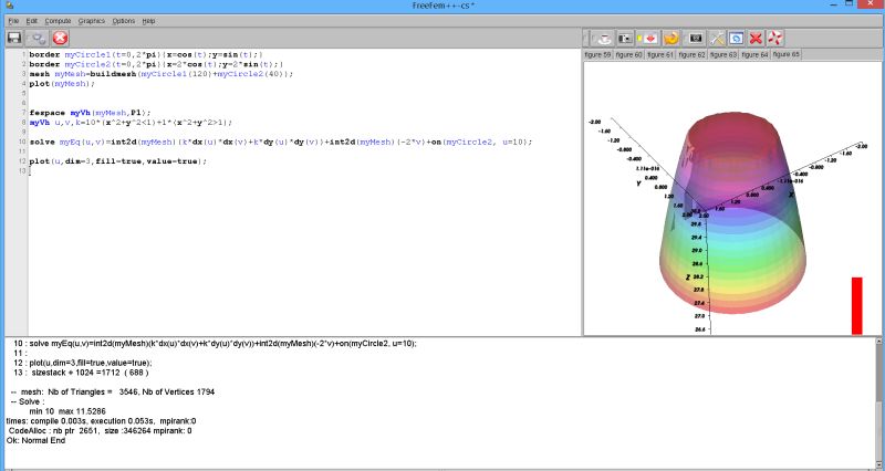
Figure 4: Solution.
Example 2 (p.1059)
Taken from an example in Lecture 21.
Lecture Note 21
Figure 5: Example from Lecture Note #19.
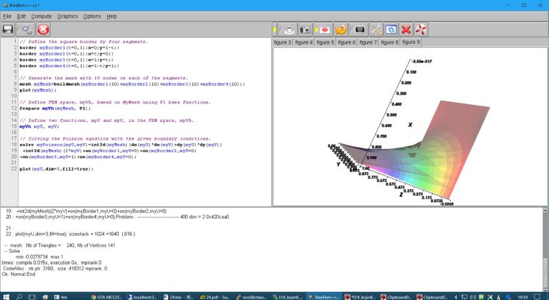
// Define the square border by four segments.
border myBorder1(t=0,1){x=0;y=1-t;};
border myBorder2(t=0,1){x=t;y=0;};
border myBorder3(t=0,1){x=1;y=t;};
border myBorder4(t=0,1){x=1-t;y=1;};

// Generate the mesh with 10 nodes on each of the segments.
mesh myMesh=buildmesh(myBorder1(10)+myBorder2(10)+myBorder3(10)+myBorder4(10));
plot(myMesh);

// Define FEM space, myVh, based on MyMesh using P1 base functions.
fespace myVh(myMesh, P1);

// Define two functions, myU and myV, in the FEM space, myVh.
myVh myU, myV;

// Solving the Poisson equation with the given boundary conditions.
solve myPoisson(myU,myV)=int2d(myMesh)(dx(myU)*dx(myV)+dy(myU)*dy(myV))
 +int2d(myMesh)(2*myV)+on(myBorder1,myU=0)+on(myBorder2,myU=0)
+on(myBorder3,myU=1)+on(myBorder4,myU=0);

plot(myU,dim=3,fill=true);
 Example 3
// Heat conduction in concentric cylinders
border myCircle1(t=0,2*pi){x=cos(t);y=sin(t);};
border myCircle2(t=0,2*pi){x=2*cos(t);y=2*sin(t);};
mesh myMesh=buildmesh(myCircle1(120)+myCircle2(40));
plot(myMesh);

fespace myVh(myMesh,P1);

// Use the boole function to define heterogeneity
myVh u,v,k=10*(x^2+y^2<1)+1*(x^2+y^2>1);

solve myEq(u,v)=int2d(myMesh)(k*dx(u)*dx(v)+k*dy(u)*dy(v))+int2d(myMesh)(-2*v)+on(myCircle2, u=10);

plot(u,dim=3,fill=true,value=true);
Figure 6: Two materials
Figure 7: Two materials
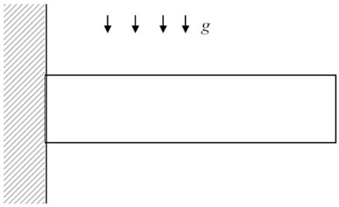
Example 4
Beam (elasticity)
- Strong form
|
μ∆ui + (μ+λ) uj,ji + bi = 0 |
|
- Weak form
|
−μ | ⌠
⌡
|
| ⌠
⌡
|
ui,jvi,j dS − (μ+λ) | ⌠
⌡
|
| ⌠
⌡
|
uj,j vj,j dS + | ⌠
⌡
|
| ⌠
⌡
|
bi vi dS = 0. |
|
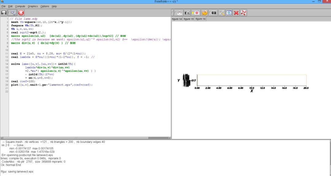
// file lame.edp
mesh Th=square(10,10,[20*x,2*y-1]);
fespace Vh(Th,P2);
Vh u,v,uu,vv;
real sqrt2=sqrt(2.);
macro epsilon(u1,u2) [dx(u1),dy(u2),(dy(u1)+dx(u2))/sqrt2] // EOM
//the sqrt2 is because we want: epsilon(u1,u2)'* epsilon(v1,v2) $== \epsilon(\bm{u}): \epsilon(\bm{v})$
macro div(u,v) ( dx(u)+dy(v) ) // EOM
real E = 21e5, nu = 0.28, mu= E/(2*(1+nu));
real lambda = E*nu/((1+nu)*(1-2*nu)), f = -1; //
solve lame([u,v],[uu,vv])= int2d(Th)(
lambda*div(u,v)*div(uu,vv)
+2.*mu*( epsilon(u,v)'*epsilon(uu,vv) ) )
- int2d(Th)(f*vv)
+ on(4,u=0,v=0);
real coef=100;
plot([u,v],wait=1,ps="lamevect.eps",coef=coef);
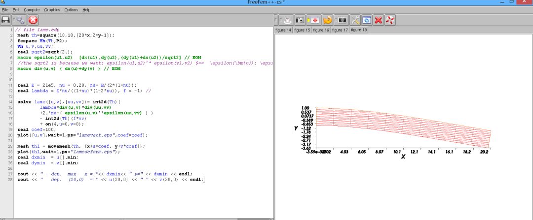
mesh th1 = movemesh(Th, [x+u*coef, y+v*coef]);
plot(th1,wait=1,ps="lamedeform.eps");
real dxmin = u[].min;
real dymin = v[].min;
cout << " - dep. max x = "<< dxmin<< " y=" << dymin << endl;
cout << " dep. (20,0) = " << u(20,0) << " " << v(20,0) << endl;
Figure 8: Beam (elasticity, before deformation)
Figure 9: Beam (elasticity, after deformation)
File translated from
TEX
by
TTH,
version 4.03.
On 18 Jan 2021, 22:29.