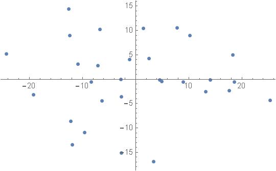
Figure 1: data points as vectors.
| (1) |
| (2) |
| (3) |
| (4) |
| (5) |
| (6) |
| Height (u) | Weight (v) | |
| 1 | 171.9 | 58.5 |
| 2 | 175.8 | 66.6 |
| 3 | 159.3 | 47.0 |
| 4 | 146.9 | 69.4 |
| 5 | 143.4 | 58.4 |
| 6 | 151.4 | 54.5 |
| 7 | 159.9 | 55.3 |
| 8 | 170.7 | 71.9 |
| 9 | 140.6 | 62.4 |
| 10 | 154.5 | 52.6 |
| 11 | 154.0 | 60.4 |
| 12 | 154.1 | 44.5 |
| 13 | 150.6 | 58.8 |
| 14 | 150.5 | 74.6 |
| 15 | 157.3 | 40.1 |
| 16 | 142.4 | 40.0 |
| 17 | 161.9 | 62.6 |
| 18 | 175.5 | 78.2 |
| 10 | 171.0 | 55.7 |
| 20 | 172.6 | 71.1 |
| 21 | 144.0 | 61.9 |
| 22 | 161.8 | 62.1 |
| 23 | 151.7 | 50.1 |
| 24 | 167.1 | 69.3 |
| 25 | 162.9 | 57.4 |
| 26 | 156.1 | 57.5 |
| 27 | 141.2 | 49.8 |
| 28 | 165.9 | 51.9 |
| 29 | 165.0 | 65.2 |
| 30 | 169.3 | 68.0 |
| Height (x) | Weight (y) | |
| 1 | 13.59 | -0.693333 |
| 2 | 17.49 | 7.40667 |
| 3 | 0.99 | -12.1933 |
| 4 | -11.41 | 10.2067 |
| 5 | -14.91 | -0.793333 |
| 6 | -6.91 | -4.69333 |
| 7 | 1.59 | -3.89333 |
| 8 | 12.39 | 12.7067 |
| 9 | -17.71 | 3.20667 |
| 10 | -3.81 | -6.59333 |
| 11 | -4.31 | 1.20667 |
| 12 | -4.21 | -14.6933 |
| 13 | -7.71 | -0.393333 |
| 14 | -7.81 | 15.4067 |
| 15 | -1.01 | -19.0933 |
| 16 | -15.91 | -19.1933 |
| 17 | 3.59 | 3.40667 |
| 18 | 17.19 | 19.0067 |
| 19 | 12.69 | -3.49333 |
| 20 | 14.29 | 11.9067 |
| 21 | -14.31 | 2.70667 |
| 22 | 3.49 | 2.90667 |
| 23 | -6.61 | -9.09333 |
| 24 | 8.79 | 10.1067 |
| 25 | 4.59 | -1.79333 |
| 26 | -2.21 | -1.69333 |
| 27 | -17.11 | -9.39333 |
| 28 | 7.59 | -7.29333 |
| 29 | 6.69 | 6.00667 |
| 30 | 10.99 | 8.80667 |
|
|

| (7) |
|
|
|
|
| # | ―x | ―y |
| 1 | 10.2536 | 8.94606 |
| 2 | 18.3264 | 4.99007 |
| 3 | -6.7595 | 10.1964 |
| 4 | -2.65911 | -15.0762 |
| 5 | -12.2102 | -8.59348 |
| 6 | -8.33284 | -0.582497 |
| 7 | -1.15698 | 4.04321 |
| 8 | 17.594 | -2.32865 |
| 9 | -11.9384 | -13.4685 |
| 10 | -7.07067 | 2.82733 |
| 11 | -2.64188 | -3.61284 |
| 12 | -12.3923 | 8.94695 |
| 13 | -6.30349 | -4.457 |
| 14 | 3.38516 | -16.9382 |
| 15 | -12.597 | 14.3837 |
| 16 | -24.3708 | 5.25141 |
| 17 | 4.9278 | -0.458496 |
| 18 | 25.2615 | -4.31341 |
| 19 | 7.81529 | 10.5906 |
| 20 | 18.5929 | -0.525273 |
| 21 | -9.57497 | -10.9737 |
| 22 | 4.54011 | -0.127296 |
| 23 | -10.817 | 3.06152 |
| 24 | 13.157 | -2.5104 |
| 25 | 2.4993 | 4.24707 |
| 26 | -2.78393 | -0.0351573 |
| 27 | -19.2559 | -3.19357 |
| 28 | 1.45742 | 10.4248 |
| 29 | 8.97179 | -0.585831 |
| 30 | 14.0826 | -0.128556 |