| |
|
|
|
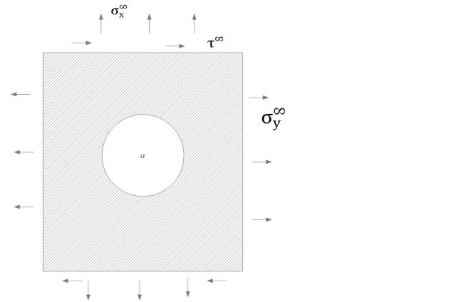
3 a4 (σx∞−σy∞) (x4−6 x2 y2+y4)
2 (x2+y2)4
|
+ |
6 a2 x2 y2 (σx∞−σy∞)
(x2+y2)3
|
+ |
a2 y4 (σx∞+σy∞)
2 (x2+y2)3
|
− |
a2 x4 (5 σx∞−3 σy∞)
2 (x2+y2)3
|
|
| |
| |
|
|
− |
4 a2 τ∞ x y (−3 a2 x2+3 a2 y2+3 x4+2 x2 y2−y4)
(x2+y2)4
|
+σx∞, |
| |
| |
|
|
|
3 a4 (σy∞−σx∞) (x4−6 x2 y2+y4)
2 (x2+y2)4
|
+ |
6 a2 x2 y2 (σy∞−σx∞)
(x2+y2)3
|
− |
a2 y4 (5 σy∞−3 σx∞)
2 (x2+y2)3
|
+ |
a2 x4 (σx∞+σy∞)
2 (x2+y2)3
|
|
| |
| |
|
|
+ |
4 a2 τ∞ x y (−3 a2 x2+3 a2 y2+x4−2 x2 y2−3 y4)
(x2+y2)4
|
+σy∞, |
| |
| |
|
|
|
τ∞ (−3 a4 x4+18 a4 x2 y2−3 a4 y4+2 a2 x6−10 a2 x4 y2−10 a2 x2 y4+2 a2 y6+x8+4 x6 y2+6 x4 y4+4 x2 y6+y8)
(x2+y2)4
|
|
| |
| |
|
| − |
a2 x y (−6 a2 σx∞ x2+6 a2 σy∞ x2+6 a2 σx∞ y2−6 a2 σy∞ y2+5 σx∞ x4−3 σy∞ x4+2 σx∞ x2 y2+2 σy∞ x2 y2−3 σx∞ y4+5 σy∞ y4)
(x2+y2)4
|
. |
| |
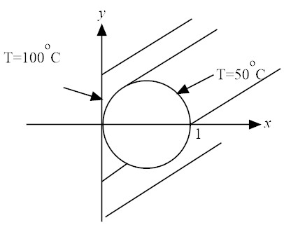 Along x=0, T=100, which is translated to a + d/y = 100. For this to be independent of y, a = 100, d = 0.
Along x2+y2−x=0, T=50, which is translated into 50=100 + c from which c=−50.
Thus, we have
Along x=0, T=100, which is translated to a + d/y = 100. For this to be independent of y, a = 100, d = 0.
Along x2+y2−x=0, T=50, which is translated into 50=100 + c from which c=−50.
Thus, we have
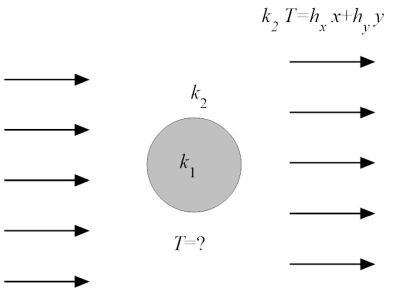
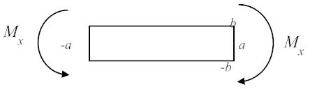
 The boundary conditions are stated as:
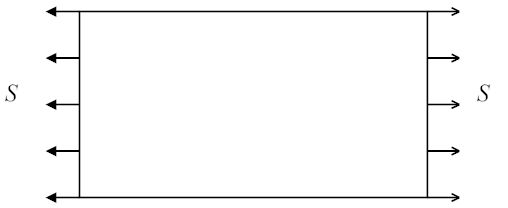
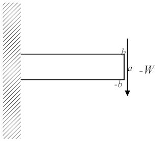
 The proper boundary conditions are stated as
 The proper boundary conditions are stated as