Discrete Fourier Transforms (DFT)

It is often necessary to obtain Fourier series applied on a set of finite data points. If one uses the conventional Fourier series expansion ¹, (1) the infinite series must be truncated and (2) numerical integration must be used to compute the Fourier coefficient, c_m, thus, introducing two layers of approximation.

The Discrete Fourier Transform (DFT) has advantages over the conventional Fourier series expansion in (1) requiring only N data points, (2) the original function can be reproduced exactly at the selected N points, (3) the coefficients of DFT do not require integration to be computed, (4) the DFT coefficients can be computed by Fast Fourier Transforms (FFT), and (5) When N is sufficiently large, DFT approaches the classical Fourier series.

FFT

The DFT coefficients are given by eq.() and are listed here again for reference

C_k =

N−1
∑
l = 0

f_l ω^−kl k = 0, 1, 2, …, (N−1).

(1)

Examples

Example 1

Consider a data set shown as

Its power spectrum (FFT) looks like

Example 2 Consider a data set of (N=10)

f₁ = {0,1,2,3,2,1,0,0,0,0 }

(2)

which looks like

The power spectrum, |C_k|², of f₁ is

Now consider

f₂={0,0,0,0,1,2,3,2,1,0}

(3)

The power spectrum, |C_k|², of f₂ is

Examples 3

Consider two different images

The power spectra of the images ² are shown as

They are identical each other even though the spatial representations are different. It can be indeed shown that the correlation between the two graphs of the power spectra is 100%.

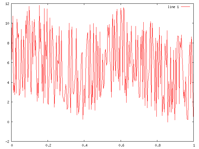
Using the fft (Fast Fourier Transform) and ifft (Inverse Fourier Transform) functions in MATLAB/OCTAVE, remove the noise from the data above and restore the original signal.

Footnotes:

f(x)=

∞
∑
m=−∞

c_m e^{i mx}, c_m =

2π

⌠
⌡

2π

0

f(x)e^−imx dx.

² The power spectrum of f(x) is defined as

|C_k|²

where

f(x) =

∑

C_k e^{i k x}.

File translated from T_EX by T_TH, version 4.03.
On 21 Aug 2022, 22:51.