 (c)
(c)
 2.
Problem
The position vector R = x i + y j to
any point in (x, y) in the x, y plane
constitutes a vector field. Draw the R vector (to scale) at
eight points that are equally spaced around the circle r = 1,
and at eight points that are equally spaced around the circle r = 3.
Solution
Easy.
3.
Problem
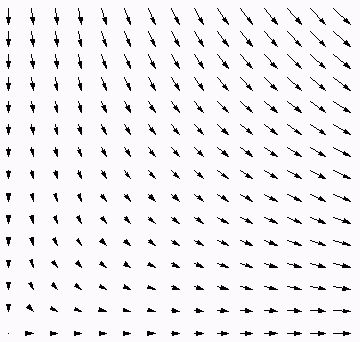
Consider the vector field v = x i − y j in
0 ≤ x ≤ ∞, 0 ≤ y ≤ ∞.
(a) On a single graph, sketch the v vectors at the 16 points (m, n),
where m and n are integers such that 0 ≤ m ≤ 3 and 0 ≤ n ≤ 3.
(Here it will help to assign a convenient scale, as we have done in Fig.4,
so that the arrow representations of the vectors will not lie on top of each other.)
2.
Problem
The position vector R = x i + y j to
any point in (x, y) in the x, y plane
constitutes a vector field. Draw the R vector (to scale) at
eight points that are equally spaced around the circle r = 1,
and at eight points that are equally spaced around the circle r = 3.
Solution
Easy.
3.
Problem
Consider the vector field v = x i − y j in
0 ≤ x ≤ ∞, 0 ≤ y ≤ ∞.
(a) On a single graph, sketch the v vectors at the 16 points (m, n),
where m and n are integers such that 0 ≤ m ≤ 3 and 0 ≤ n ≤ 3.
(Here it will help to assign a convenient scale, as we have done in Fig.4,
so that the arrow representations of the vectors will not lie on top of each other.)
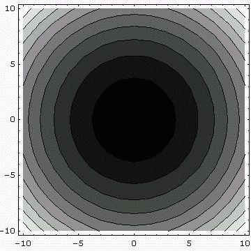
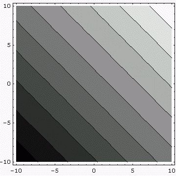
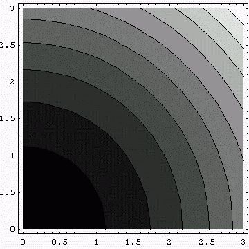
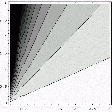
 (b) Determine the curves along which v has constant magnitude and
those along which v
has constant direction. Are these results in agreement with your sketch of
the field in part (a)?
Solution
Constant magnitude: x2 + y2 = const.
(b) Determine the curves along which v has constant magnitude and
those along which v
has constant direction. Are these results in agreement with your sketch of
the field in part (a)?
Solution
Constant magnitude: x2 + y2 = const.
 Constant direction:
|
|
|
|
|
|
|
|
|
|
|
|
|
|
|
| (L'Hospital's theorem) |
|
|
|
|
|
|
|
|
|
|
|
|
|
|
|
| (3) |
| (4) |
| (5) |
|
|
|
|
|
|
|
|
| (13) |
|
|
|
|
|
|
|
|
|
|
|
|
|
|
| (18) |
| (19) |
| (20) |
| (21) |
|
|
|
|
|
|
|
|
|
|
|
|
|
|
|
|
|
|
|
|
|
|
|
|
|
|
|
|
|
|
|
|
|
|
|
|
|
|
|
|
|
|
|
|
|
|
|
|
|
|
|
|
|
|
|
|
|
|
| (63) |
| (64) |
|
| (67) |
|
|
|
|
|
|
|
|
|
|
|
|
|
|
|
|
|
| (80) |
| (81) |
| (82) |
| (83) |
| (84) |
|
|
| (87) |
| (88) |
|
|
| (94) |
|
|
|
|
|
|
|
|
|
|
|
|
|
|
|
| (111) |
| (112) |
| (113) |
|