#25 (11/29/2023)

Wavelet transforms

Fourier series

In the Fourier series, the Fourier coefficients, C_m, do not contain any information on x

f(x) =

∞
∑
m = − ∞

C_m e^{i m x}, C_m =

2π

⌠
⌡

∞

−∞

f(x) e^{− i m x} d x.

(1)

=		×a₁
+		×a₂
+		×a₃
+		×a₄

Multi-resolution decomposition

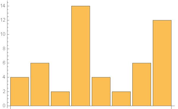
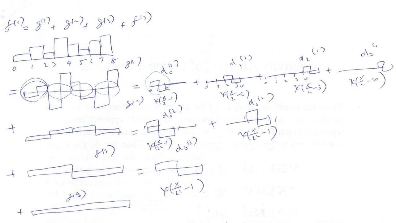
f⁽⁰⁾(x)={4,6,2,14,4,2,6,12}

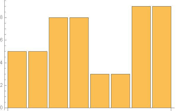
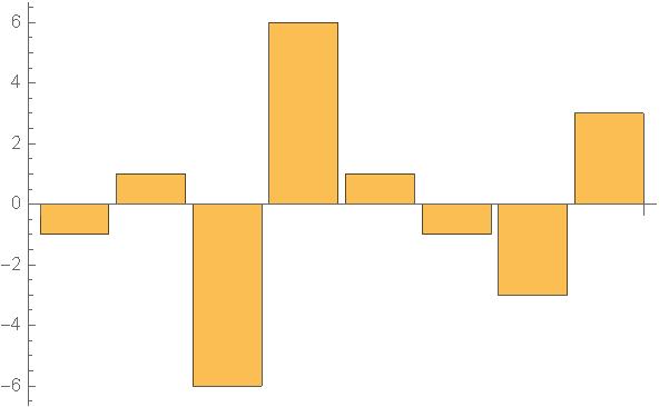
f⁽¹⁾(x)={5,8,3,9}	g⁽¹⁾(x)={−1,−6,1,−3}
	+

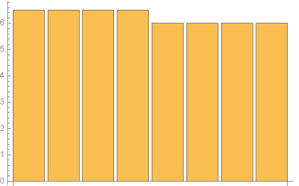
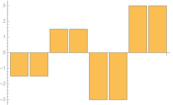
f⁽²⁾(x)={6.5, 6.0}	g⁽²⁾(x)={−1.5,−3.0}
	+

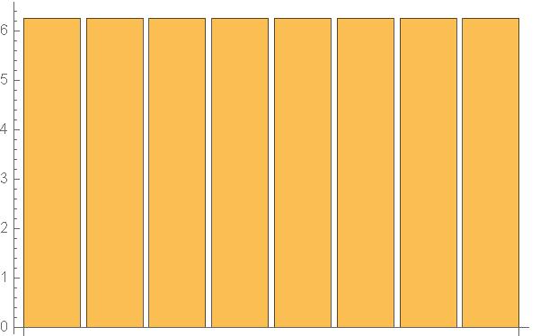
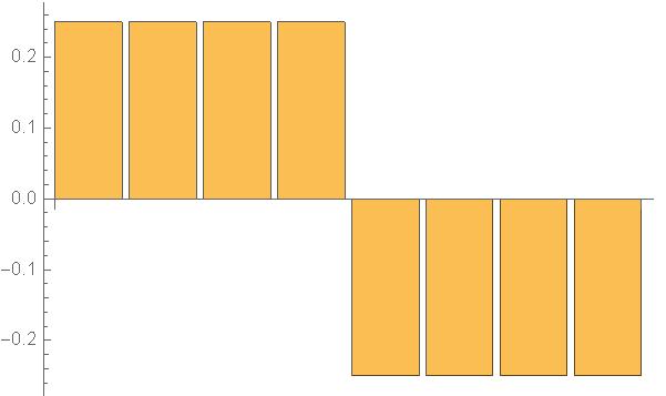
f⁽³⁾(x)={6.25}	g⁽³⁾(x)={0.25}
	+

Multiresolution analysis (Wavelet transforms)

A function, f⁽⁰⁾(x), is defined as a discrete data set as

f⁽⁰⁾(x) =

⎧
⎪
⎪
⎨
⎪
⎪
⎩

c₀

0 ≤ x < 1

c₁

1 ≤ x < 2

c_N−1

N − 1 ≤ x < N

(2)

where N = 2ⁿ.

The next level (scale 2) of f⁽⁰⁾(x), f⁽¹⁾(x) can be defined by replacing two consecutive terms by their averages as

f⁽¹⁾(x) =

⎧
⎪
⎪
⎨
⎪
⎪
⎩

c₀⁽¹⁾

(=(c_o+c₁)/2)

0 ≤ x < 2

c₁⁽¹⁾

(=(c₁+c₂)/2)

2 ≤ x < 4

c_N/2−1⁽¹⁾

(=(c_N−2+c_N−1)/2)

N − 2 ≤ x < N

(3)

An interval where the values remain the same is called a scale. The function, f⁽⁰⁾(x) is a function of scale 1 and the function f⁽¹⁾(x) is a function of scale 2.

The function with scale 4 is thus defined by

f⁽²⁾(x) =

⎧
⎪
⎪
⎨
⎪
⎪
⎩

c₀⁽²⁾

(=(c⁽¹⁾_o+c⁽¹⁾₁)/2)

0 ≤ x < 4

c₁⁽²⁾

(=(c⁽¹⁾₁+c⁽¹⁾₂)/2)

2 ≤ x < 8

c_N/4−1⁽²⁾

(=(c⁽¹⁾_N/2−2+c⁽¹⁾_N/2−1)/2)

N − 4 ≤ x < N

(4)

Finally, the function of scale N is

f⁽ⁿ⁾(x) = c⁽ⁿ⁾₀

⎛
⎝

c⁽ⁿ⁻¹⁾₀ + c⁽ⁿ⁻¹⁾₁

⎞
⎠

, 0 ≤ x < N,

(5)

which is the entire average of f⁽⁰⁾(x).

The inverse of scale is called resolution.

Multi-resolution decomposition

Let the difference between the function of scale 1, f⁽⁰⁾(x), and the function of scale 2, f⁽¹⁾(x), be denoted as g⁽¹⁾(x) as

f⁽⁰⁾(x) = g⁽¹⁾(x) + f⁽¹⁾(x).

(6)

Similarly,

f⁽¹⁾(x) = g⁽²⁾(x) + f⁽²⁾(x).

(7)

and

f⁽ⁿ⁻¹⁾(x) = g⁽ⁿ⁾(x) + f⁽ⁿ⁾(x).

(8)

Therefore, f⁽⁰⁾(x) can be decomposed as

f⁽⁰⁾(x)

g⁽¹⁾(x) + f⁽¹⁾(x)

(9)

g⁽¹⁾(x) + g⁽²⁾(x) + f⁽²⁾(x)

(10)

g⁽¹⁾(x) + g⁽²⁾(x) + g⁽³⁾(x) +f⁽³⁾(x)

(11)

(12)

g⁽¹⁾(x) + g⁽²⁾(x) + g⁽³⁾(x) + g⁽⁴⁾(x) + …+ g⁽ⁿ⁾(x) + f⁽ⁿ⁾(x).

(13)

This decomposition is called multiscale decomposition which looks similar to Fourier series. However, the amplitude of each component in the Fourier series is uniform while the amplitude of g⁽ⁱ⁾(x) varies.

Scaling Functions

The Haar scaling function, ϕ(x), is defined as

ϕ(x) =

⎧
⎪
⎨
⎪
⎩

0 ≤ x < 1

otherwise

(14)

The function, ϕ(x), above is a function with [0, 1) as a support. Using ϕ(x), the function of scale 1, f⁽⁰⁾(x), can be expressed as

f⁽⁰⁾(x) =

N−1
∑
k=0

c_k⁽⁰⁾ ϕ(x − k), c_k⁽⁰⁾ = c^k.

(15)

The function of scale 2, f⁽¹⁾(x), can be expressed as

f⁽¹⁾(x) =

N/2−1
∑
k=0

c_k⁽¹⁾ ϕ(x/2 − k), c_k⁽¹⁾ =

c⁽⁰⁾_2k+c⁽⁰⁾_2k+1

(16)

The function of scale 4, f⁽²⁾(x), can be expressed as

f⁽²⁾(x) =

N/4−1
∑
k=0

c_k⁽²⁾ ϕ(x/4 − k), c_k⁽²⁾ =

c⁽¹⁾_2k+c⁽¹⁾_2k+1

(17)

In general, the function of scale 2^j can be expressed as

f^(j)(x) =

N/2^j−1
∑
k=0

c_k^(j) ϕ(x/2^j − k), c_k^(j) =

c^(j−1)_2k+c^(j−1)_2k+1

(18)

The number, j, when the scale is 2^j is called a level.

Orthogonality

The inner product over [0, N) between p(x) and q(x) is define as

(p, q) =

⌠
⌡

N

0

p(x) q(x) dx,

(19)

If we define

ϕ^(j)_k(x) ≡ ϕ

⎛
⎝

2^j

− k

⎞
⎠

(20)

it follows

(ϕ_k^(j), ϕ^(j)_k′) =

⌠
⌡

N

0

ϕ_k^(j) (x) ϕ_k′^(j) dx = 0, k ≠ k′.

(21)

For each level, j, a linear space spanned by ϕ^(j)_k(x) is denoted as V^(j). The space, V^(j), is a linear space of N/2^j dimensions with ϕ^(j)_k(x) as the orthogonal bases.

V⁽⁰⁾ ⊃ V⁽¹⁾ ⊃ V⁽²⁾ ⊃ … ⊃ V⁽ⁿ⁾

(22)

Wavelet

The Haar wavelet mother function is defined as

ψ(x) =

⎧
⎪
⎨
⎪
⎩

0 ≤ x < 1/2

−1

1/2 ≤ x < 1

otherwise

(23)

This is a function with [0, 1) as a support. Using this function, the function of scale 1, g⁽¹⁾(x), can be written as

g⁽¹⁾(x)

f⁽⁰⁾(x) − f⁽¹⁾(x)

(24)

⎧
⎪
⎪
⎪
⎨
⎪
⎪
⎪
⎩

c₀⁽⁰⁾ − (c₀⁽⁰⁾ + c₁⁽⁰⁾)/2

0 ≤ x < 1

c₁⁽⁰⁾ − (c₀⁽⁰⁾ + c₁⁽⁰⁾)/2

1 ≤ x < 2

c₂⁽⁰⁾ − (c₂⁽⁰⁾ + c₃⁽⁰⁾)/2

2 ≤ x < 3

c_N−2⁽⁰⁾ − (c_N−2⁽⁰⁾ + c_N−1⁽⁰⁾)/2

N−2 ≤ x < N−1

c_N−1⁽⁰⁾ − (c_N−2⁽⁰⁾ + c_N−2⁽⁰⁾)/2

N−1 ≤ x < N

(25)

⎧
⎪
⎪
⎪
⎪
⎨
⎪
⎪
⎪
⎪
⎩

(c₀⁽⁰⁾ − c₁⁽⁰⁾)/2

0 ≤ x < 1

− (c₀⁽⁰⁾ − c₁⁽⁰⁾)/2

1 ≤ x < 2

(c₂⁽⁰⁾ − c₃⁽⁰⁾)/2

2 ≤ x < 3

− (c₂⁽⁰⁾ − c₃⁽⁰⁾)/2

3 ≤ x < 4

(c_N−1⁽⁰⁾ − c_N−2⁽⁰⁾)/2

N−2 ≤ x < N−1

− (c_N−1⁽⁰⁾ − c_N−2⁽⁰⁾)/2

N−1 ≤ x < N

(26)

N/2−1
∑
k=0

d_k⁽¹⁾ ψ

⎛
⎝

−k

⎞
⎠

(27)

where

d_k⁽¹⁾ ≡

c⁽⁰⁾_2k − c⁽⁰⁾_2k+1

(28)

In general,

g^(j)(x) =

N/2^j−1
∑
k=0

d_k^(j) ψ

⎛
⎝

2^j

−k

⎞
⎠

(29)

where

d_k^(j) ≡

c^(j−1)_2k − c^(j−1)_2k+1

(30)

The wavelet of level j and position k is defined as

ψ_k^(j)(x) ≡ ψ

⎛
⎝

2^j

−k

⎞
⎠

(31)

For each level, j, the wavelet functions, {ψ_k^(j)(x)}, k = 0, …, N/2^j−1 are orthogonal, i.e.,

(ψ_k^(j), ψ_k′^(j)) =

⌠
⌡

N

0

ψ_k^(j)(x) ψ_k′^(j)(x) dx = 0, k ≠ k′.

(32)

Using the wavelet function, f⁽⁰⁾(x), can be expressed as

f(x)

N/2−1
∑
j=1

g^(j)(x) + f⁽ⁿ⁾(x)

(33)

N/2−1
∑
j=1

N/2^j−1
∑
k=1

d_k^(j) ψ

⎛
⎝

2^j

− k

⎞
⎠

+ f⁽ⁿ⁾(x)

(34)

N/2−1
∑
j=1

N/2^j−1
∑
k=1

d_k^(j) ψ^j_k(x) + f⁽ⁿ⁾(x),

(35)

where

ψ^j_k(x) ≡ ψ

⎛
⎝

2^j

− k

⎞
⎠

which is called the wavelet of level j and position k.

Continuous wavelet

The wavelet transform for continous function, f(x), can be defined as

W(b, a) ≡

√a

⌠
⌡

∞

−∞

f(x)

⎛
⎝

x − a

⎞
⎠

d x

(36)

where ―ψ(x) is the complex conjugate of a mother wavelet, ψ(x).

The inverse wavelet transform can be defined as

f(x) ≡

C_ψ

⌠
⌡

∞

−∞

⌠
⌡

∞

−∞

W(b,a)

√a

⎛
⎝

x − a

⎞
⎠

a²

d b,

(37)

where

C_ψ ≡

⌠
⌡

∞

−∞

|ψ(ω)|²

|ω|

d ω.

Some examples

source

File translated from T_EX by T_TH, version 4.03.
On 27 Nov 2023, 19:25.