#21 (11/18/2024)

Laplace transforms

Formulae of the Fourier transform1 and the inverse Fourier transform are listed here for reference as

F(x)
=
1


−∞ 

F
 
(ω) ei ωx dω,

F
 
(ω)
=


−∞ 
F(x) ei ωx dx.
(1)
The Laplace transform can be derived as a special case of the Fourier transforms by limiting the range of f(x) over (0, ∞). By combining Eq. (1) and Eq. (1), one obtains
F(x) = 1

2 π


−∞ 


−∞ 
F(y) ei ωy dy
ei ωx dω.
(2)
laplace1.jpg
If we require that

F(x) =


e−γx f(x)
    x > 0
0
    x < 0,
(3)
where γ is a positive number (to ensure that F(x) → 0 as x→ ∞), then for x > 0,

e−γx f(x)
=
1

2 π


−∞ 


−∞ 
F(y) ei ωy dy
eiωx dω
=
1


−∞ 


0 
f(y) e−(γ+ iω) y dy
eiωx dω.
(4)
For x > 0, multiplying eγx on the both sides of Eq. (4) yields

f(x) = 1

2 π


−∞ 


0 
f(y) e−(γ+iω) y dy
e(γ+ i ω)x dω.
(5)
If we let
γ+ i ω ≡ s,
then
i dω = ds,
so that Eq. (5) becomes
f(x)
=
1


γ+ i

γ−i 


0 
f(y) es y dy
esx ds

i
=
1

i

γ+ i

γ− i 
-
f
 
(s) es x ds,
(6)
where
-
f
 
(s) ≡


0 
f(x)es x dx.
(7)
s-plane.jpg
Equation (7) is called the Laplace transform of f(x) and Eq. (6) is called the inverse Laplace transform.
As discussed in class, the Laplace transforms are special cases of the Fourier transforms by restricting F(t) 
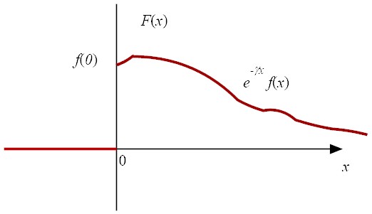
2 to exp(−γt) f(t) for t > 0, 
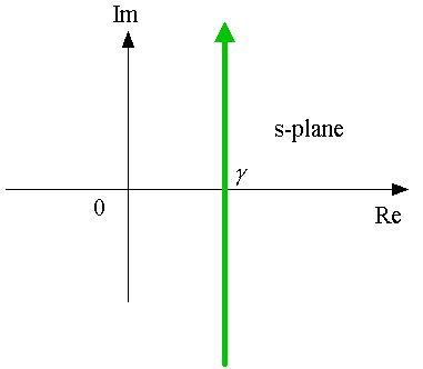
where γ is a positive number. For the convergence of the Laplace transform, f(t) must be a function such that e−γt f(t) → 0 as t→ ∞ for an appropriately chosen positive value of γ. Such functions include

f(t) = 1
Choose γ = 1,
(8)
f(t) = t
Choose γ = 1,
(9)
f(t) = t100
Choose γ = 1,
(10)
f(t) = e100t
Choose γ = 101,
(11)
but not
f(t) = exp (t2),
(12)
as it is not possible to choose γ such that e−γt exp(t2) vanishes as t→ ∞.

Properties of Laplace transforms


    (1) Linearity
    Lf + βg) = αL (f) + βL (g).
    (13)

    (2) Differentiation
    L f(n) = sL f(n−1)f(n−1) (0).
    (14)
    (Proof): For n=1,

    L(f′)
    =


    0 
    f′(t) est dt
    =
    [ f(t) est]0


    0 
    f(t) (−s) es t dt
    =
    fest|fest|0 +s


    0 
    f(t) est dt
    =
    s L(f) − f(0)
    =
    s
    -
    f
     
    (s) − f(0).
    (15)
    Use mathematical induction to complete the proof.
    For n = 2,

    L(f  "(t))
    =
    s L(f  ′(t)) − f  ′(0)
    =
    s
    s
    -
    f
     
    (s) − f(0)
    f  ′(0)
    =
    s2
    -
    f
     
    (s) − s f(0) − f  ′(0).
    (16)


    (3) Laplace convolution theorem
    The Laplace convolution is defined as

    f * g =
    t

    0 
    f(t − τ) g(τ) dτ.
    (17)
    Note that the integral range is different from that in the Fourier convolution.
    Note also
    f * g = g * f.

    The Laplace convolution theorem is stated as
    L (f * g) =
    -
    f
     
    (s)
    -
    g
     
    (s).
    (18)
(Proof):
L

t

0 
f(t − τ) g(τ) d τ
=


0 


t

0 
f(t − τ) g(τ) d τ
es t d t
=


0 


τ 
f(t − τ) es t d t
g(τ) d τ
=


0 


0 
f(p) es (τ+ p) d p
g(τ) dτ
=


0 


0 
f(p) es p d p es τ
g(τ) dτ
=


0 


0 
f(p) es p d p
g(τ) es τ d τ
=


0 
f(p) es p d p  


0 
g(τ) es τ d τ
=
-
f
 
(s)  
-
g
 
(s),
(19)
where the order of integrations was changed.
convproof.jpg

τ
:
0 → t
t
:
0 → ∞

t
:
τ→ ∞
τ
:
0 → ∞

Some important Laplace transforms


t
s
ta
Γ(a + 1)

sa + 1
3
ea t
1

sa
sin at
a

s2 + a2
cos at
s

s2 + a2
H(ta)
exp(−a s)

s
sinh at
a

s2a2
cosh at
s

s2a2
eat f(t)
-
f
 
(s+a)
(20)
You can verify the above by the following forms:
Laplace transform
Enter the function to be Laplace transformed.
with respect to .

Example:
t^4 (must be lowercase t) t

Inverse Laplace transform
Enter the function to be inverse Laplace transformed.
with respect to .

Example:
1/(s^2+4) (must be lowercase s)


Example 1 (initial value problem)

⋅⋅
x
 
(t) + x(t) = f(t),
(21)
with x(0) and · x(0) are given as the initial conditions.
Equation (21) can be Laplace transformed to

s2
-
x
 
s x(0) −

x
 
(0) +
-
x
 
=
-
f
 
(s),
(22)
which can be solved as

-
x
 
=
-
f
 
(s)

1 + s2
+

x
 
(0)

1 + s2
+ s

1 + s2
x(0).
(23)
The inverse Laplace transform of eq.(23) is

x(t)
=
f(t) * sin t +

x
 
(0) sin t + x(0) cos t
=

t

0 
f(t−τ) sin τdτ+

x
 
(0) sin t + x(0) cos t.
(24)
Note that the convolution theorem was used.
Example 2
Simultaneous differential equations:


dx

dt
= x + y,     x(0)=1,
dy

dt
= 4 x + y,     y(0)=0.
(25)
(Solution): Because of the way the initial condition is given at t=0 and the range of t is (0, ∞), the Laplace transform should be used. By transforming each equation into the s domain, one obtains

s
-
x
 
(s) − x(0)
=
-
x
 
(s) +
-
y
 
(s)
(26)
s
-
y
 
(s) − y(0)
=
4
-
x
 
(s) +
-
y
 
(s)
(27)
which can be solved as

-
x
 
(s)
=
s−1

(s−1)2−4
(28)
-
y
 
(s)
=
4

(s−1)2−4
(29)
From the table above, one can find
x(t)
=
et cosh 2t
(30)
y(t)
=
2 et sinh 2t.
(31)
Inverse Laplace transform
Enter the function to be inverse Laplace transformed.
with respect to .
Alternatively,
x(t)= s−1

(s+1)(s−3)
= 1

2(s−3)
+ 1

2(s+1)
,
(32)

y(t)= 4

(s+1)(s−3)
= 1

s−3
1

s+1
.
(33)
Therefore,
x(t) = 1

2
e3t + 1

2
et, .    y(t)=e3tet.
(34)

Partial fraction


P(s)

(sa1)m1 (sa2)m2 …(san)mn
= A0+A1 s + A2 s2 + …Am1−1sm1−1

(sa1)m1
+…
(35)

Example:
s+1

s3 (s+2)
= a0+a1s + a2 s2

s3
+ b0

s+2
.
(36)
In order to determine the unknowns, the denominators can be eliminated as

s + 1 = (a0+a1s + a2 s2)(s+2) + b0 s3.
(37)

s = −2
−1 = −8 b0,
(38)
s = 0
1 = 2 a0.
(39)
To obtain two more conditions (four unknowns !), eq.(37) can be differentiated as

1 = (a1 + 2a2 s) (s+2) + (a0 + a1 s + a2 s2) + 3 b0 s2.
(40)

s = 0
1 = 2 a1 + a0.
(41)
Differentiating eq.(40) again as

0 = 2a2 (s+2)+ (a1 + 2a2 s) + (a1 + 2a2 s)+ 6 b0 s,
(42)

s = 0
0 = 4 a2 + a1+a1,
(43)
so

b0= 1

8
,     a0= 1

2
,     a1= 1

4
,     a2=− 1

8
.
(44)

s+1

s3 (s+2)
=

1

2
+ s

4
s2

8


s3
+

1

8


s+2
=
1

2s3
+ 1

4s2
1

8s
+ 1

8 (s+2)
.
(45)

Additional Laplace transforms table


t
s
d

dt
f(t)
s
-
f(s)
 
f(0)
t f(t)
d

ds
-
f
 
(s)
tn f(t)
(−1)n dn

dsn
-
f
 
(s)
1

t
f(t)


s 
-
f
 
(s) ds

t

0 
f(t) dt
1

s
-
f
 
(s)
H(ta) f(ta)
es a
-
f
 
(s)
ea t f(t)
-
f
 
(sa)
(46)
It is roughly noted from the table above that multiplying by es (or et) has a shifting effect in the transformed domain, multiplying by t (or s) is translated into differentiation in the transformed domain and division by t (or s) is translated into integration in the transformed domain. With a proper combination of the entries above combined with the Laplace convolution theorem, it is possible to bypass the formula of the inverse Laplace transform all together.

More exercise problems

  1. Solve the following differential equation:

    ⋅⋅
    y
     
    (t) + y(t) = sin t,     y(0)  and

    y
     
    (0)   given.
    (47)
    (Solution) Laplace transforms of the both sides yield:

    s2
    -
    y
     
    (s) − s y(0) −

    y
     
    (0) +
    -
    y
     
    (s) = 1

    1+s2
    ,
    (48)
    which can be solved for y(s) as
    -
    y
     
    (s) = 1

    (1+s2)2
    + s

    1+s2
    y(0) + 1

    1+s2

    y
     
    (0).
    (49)
    Hence, the inverse of the above is
    y(t)
    =
    sin t*sin t + y(0) cos t +

    y
     
    (0) sin t
    =

    t

    0 
    sin (t − τ) sin τ dτ4 + y(0) cos t +

    y
     
    (0) sin t
    =
    1

    2
    (−t cos t +sin t) + y(0) cos t +

    y
     
    (0) sin t.
    (50)

  2. Solve the following integral equation.
    y(t) = t +
    t

    0 
    sin (t − τ) y(τ) dτ.
    (51)
    (Solution) Laplace transform the both sides of the equation to get
    -
    y
     
    = 1

    s2
    + 1

    s2 + 1
    -
    y
     
    ,
    (52)
    from which it follows
    -
    y
     
    = s2 + 1

    s4
    = 1

    s2
    + 1

    s4
    ,
    (53)
    which can be inverted to yield
    y(t) = t + t3

    6
    .
    (54)
  3. Prove

    lim
    s → ∞ 
    s
    -
    f
     
    (s) = f(0).
    (Solution) Use the definition,
    L(f  ′(t))
    =


    0 
    f′(t) es t d t
    =
    s  
    -
    f
     
    (s) − f(0),
    (55)
    and let s → ∞.
  4. Prove

    lim
    s → ∞ 
    -
    f
     
    (s) = 0.
    (Solution)
    Use the definition,
    L(f(t))
    =


    0 
    f(t) es t d t
    =
    -
    f
     
    (s),
    (56)
    and let s → ∞.
  5. Find the inverse Laplace transform for
    1

    (s + 3)4
    .
    (Solution)
    From
    L(t3) = 3!

    s4
    ,     L(ea t f(t)) =
    -
    f
     
    (sa),

    L−1
    1

    (s + 3)4

    = e−3 t t3

    3!
    .
  6. Find the inverse Laplace transform for
    s + 2

    s3 (s − 1)
    .
    (Solution) Use partial fraction to get
    s + 2

    s3 (s − 1)
    =
    3

    s − 1
    2 + 3 s + 3 s2

    s3
    =
    3

    s − 1
    − − 3

    s
    3

    s2
    2

    s3
    ,
    (57)
    so

    L−1
    s + 2

    s3 (s − 1)

    = 3 et −3 − 3 tt2.
  7. Express the Laplace transform for
    t f′(t).
    (Solution)
    Note that L(t f(t)) = −[(d)/(ds)] f(s). Therefore,
    L(t f′(t)) = − d

    ds
    L(f′(t)) = − d

    ds

    s
    -
    f
     
    (s)−f(0)
    = −

    -
    f
     
    (s)+ s
    d
    -
    f
     
    (s)

    ds


    .
  8. Solve the diffusion equation,
    u

    t
    = 2 u

    x2
    ,
    with
    u = 0   at   t = 0,     u = 0   at   x = 0,     u = 100   at   x = 1.
    by the Laplace transform.
    (Solution) Laplace transform the original equation with respect to t to get
    s
    -
    u
     
    =
    d2
    -
    u
     

    d x2
    ,
    which can be solved for u as
    -
    u
     
    = A es x + B e− √s x.
    The boundary conditions are
    -
    u
     
    |x = 0 = A + B = 0,

    -
    u
     
    |x = 1 = A es + B e−√s = 100

    s
    ,
    which can be solved for A and B as
    A = 100

    s (ese−√s)
    ,    B = − 100

    s (ese−√s)
    .
    Therefore,
    -
    u
     
    = 100

    s
    esxe−√s x

    ese−√s
    The inverse of u needs to wait for the spring semester (ME5332).

Z-transform

If f(t) takes only discrete values, f0, f1, f2, f3 ... at t = 0, 1, 2, 3, …n as
f(t) ≡

n=0 
fn δ(tn),
(58)
its Laplace transform is
L(f(t))
=


0 
f(t) es t dt
=


0 


n=0 
fn δ(tn)
es t dt
=


n=0 
fn


0 
δ(tn) es t dt
=


n=0 
fn

(es)n
=


n=0 
fn

zn
,
(59)
where
zes.
(60)
Equations (59) is called the Z-transform of fn and is denoted by

Z(fn) =
-
f
 
(z) =

n=0 
fn

zn
.
(61)
The inverse Z-transform can be computed as (proof skipped)

fn = Z−1(
-
f
 
(z)) = 1

2 πi

(⎜)

-
f
 
(z) zn−1 dz,
(62)
where the integral path (in the complex plane) is a closed loop that contains all the poles of Z(an) (for details, wait until you take ME5332).
Laplace transform:

t
s
f(t)
-
f
 
(s)=


0 
f(t)est ds
(63)

Z-transform


n
z
fn
-
f
 
(z) =

n=0 
fn zn
(64)
As the Z-transform is a special case of the Laplace transform, similar properties to those for the Laplace transform hold:

    (1) Linearity
    Zfn + βgn) = αZ(fn) + βZ(gn).

    (2) Shift (equivalent to derivative)
    Z(fn+1) = z
    -
    f
     
    (z) − z f0.
    (Proof)
    Z(fn+1)
    =


    n=0 
    fn+1

    zn
    =
    z

    n=0 
    fn+1

    zn+1
    =
    z

    n=1 
    fn

    zn
    =
    z


    n=0 
    fn

    zn
    f0
    =
    z
    -
    f
     
    (z) − z f0.
    (65)
    Note that
    Z(fn+2)
    =
    z Z(fn+1) − z f1
    =
    z
    z
    -
    f
     
    (z)−z f0
    z f1
    =
    z2
    -
    f
     
    (z) − z2 f0z f1.
    (66)

    (3) Convolution theorem

    Z(fn * gn) =
    -
    f
     
    (z)
    -
    g
     
    (z),
    where
    fn*gn n

    m=0 
    fnm gm.
Just like the Laplace transform is useful for an initial value problem in differential equations, the Z-transform is useful for difference equations.

fn
z
1
z

z−1
n
z

(z−1)2
n2
z (z+1)

(z−1)3
n3
z (z2+4 z+1)

(z−1)4
n4
z (z3+11 z2+11 z+1)

(z−1)5
an
z

za
sin n
z sin(1)

z2−2 z cos(1)+1
cos n
z (z−cos(1))

z2−2 z cos(1)+1
fn+1
z
-
f
 
(z) − z f0
fn+2
z2
-
f
 
(z) − z2 f0z f1
(67)
Example
(Fibonacci numbers)
davinci-fibonacci.jpg from Da Vinci Code
Find the general form of fn that satisfies

fn+2 = fn+1 + fn,     f0 = 1,   f1 = 1.
(Solution)

Apply the Z-transform on the difference equation to get

z
z
-
f
 
(z) − z f0
z f1
=
(z
-
f
 
(z) − z f0) +
-
f
 
(z),
(68)
z2
-
f
 
(z) − z2z
=
z
-
f
 
(z) − z +
-
f
 
(z),
(69)
which can be solved as

-
f
 
(z) = z2

z2z − 1
.
(70)
Noting that
z2

z2z − 1
= α

α− β
z

z − α
β

α− β
z

z − β
,
(71)
where
α = 1 + √5

2
,     β = 1 − √5

2
.
Equation (70) can be inverse Z-transformed using the table above as:

fn = α

α− β
αn β

α− β
βn.
(72)
Alternatively try this:
Enter the function to be inverse z-transformed.
with respect to .


fn = −

1

2
√5

2

n

 
(−5 + √5) +
1

2
+ √5

2

n

 
(5 + √5)

10
.
(73)


Footnotes:

1One of the three definitions. This is derived from Fourier series.
2 Because the variable used in the Laplace transform is often time, "t" is customarily used instead of "x."
3
Γ(s) ≡


0 
ts − 1 et d t,     Γ(n) = (n − 1)!     n: integer
4 Note that
sin (t − τ) sin τ = 1

2
(cos (t−2 τ) − cos t)
so

t

0 
cos (t−2 τ) dτ = sin t,    
t

0 
cos t dτ = t cos t.


File translated from TEX by TTH, version 4.03.
On 16 Nov 2024, 15:56.