| |
|
|
| ⌠
⌡
|
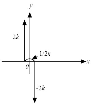
0
−1/(2k)
|
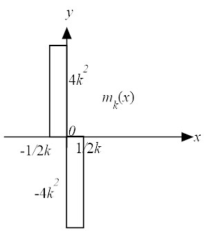
4 k2 f(x)dx + | ⌠
⌡
|
1/(2k)
0
|
(−4 k2) f(x)dx |
| |
| |
|
|
4k2 | ⌠
⌡
|
0
−1/(2k)
|
f(x)dx −4k2 | ⌠
⌡
|
1/(2k)
0
|
f(x)dx |
| |
| |
|
|
4k2 | ⌠
⌡
|
0
−1/(2k)
|
| ⎛
⎝
|
f(0)+ f′(0) x + |
f"(0)
2!
|
x2 + |
f"′(0)
3!
|
x3 + … | ⎞
⎠
|
dx |
| |
| |
|
|
−4 k2 | ⌠
⌡
|
1/(2k)
0
|
| ⎛
⎝
|
f(0)+ f′(0) x + |
f"(0)
2!
|
x2 + |
f"′(0)
3!
|
x3 + … | ⎞
⎠
|
dx |
| |
| |
|
|
4k2 | ⎛
⎝
|
|
f(0)
2k
|
− |
f′(0)
8 k2
|
+ |
f"(0)
48 k3
|
− |
f"′(0)
384 k4
|
+… | ⎞
⎠
|
−4k2 | ⎛
⎝
|
|
f(0)
2k
|
+ |
f′(0)
8 k2
|
+ |
f"(0)
48 k3
|
+ |
f"′(0)
384 k4
|
+… | ⎞
⎠
|
|
| |
| |
|
|
−f′(0) − |
f"′(0)
48
|
|
1
k2
|
− … |
| |
| |
|
| | (8) |