#18 (11/03/2025)
Note
Fourier coefficients (integrals) are pseudo-symmetric with respect to m or ω as
Proof.
Just use the definition.
Power spectrum is symmetrical, i.e.
Proof.
Just use the definition.
Nyquist-Shannon Sampling theorem
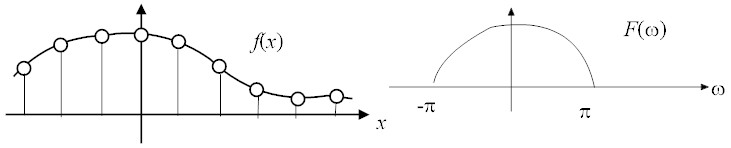 A Fourier transformable function, f(x), can be completely represented by
its discrete values at x = …−3, 2, 1, 0, 1, 2, … by
A Fourier transformable function, f(x), can be completely represented by
its discrete values at x = …−3, 2, 1, 0, 1, 2, … by
| |
|
|
…+ f(−1) |
sin π(x + 1)
π(x + 1)
|
+f(0) |
sin πx
πx
|
+f(1) |
sin π(x − 1)
π(x − 1)
|
+ … |
| |
| |
|
|
∞
∑
k=−∞
|
f(k) |
sin π(x−k)
π(x−k)
|
|
| | (4) |
|
if f(x) does not contain higher frequency components than π, i.e.
Proof
As the bandwidth of f(x) is restricted between −π < ω < π, the inverse
Fourier transform of f(x) is
|
f(x) = |
1
2 π
|
| ⌠
⌡
|
∞
−∞
|
F(ω) ei ωx dω = |
1
2 π
|
| ⌠
⌡
|
π
−π
|
F(ω) ei ωx dω, |
| (5) |
where
|
F(ω) = | ⌠
⌡
|
∞
−∞
|
f(x) e−iωx dx. |
|
As F(ω) exists only in the interval [−π, π], it can be
expressed by the Fourier series as
|
F(ω) = |
∞
∑
k=−∞
|
Ck ei k ω, |
| (6) |
where
| |
|
|
|
1
2 π
|
| ⌠
⌡
|
π
−π
|
F(ω) e−i k ω dω |
| |
| |
|
|
|
1
2 π
|
| ⌠
⌡
|
π
−π
|
F(ω) ei ω(−k) dω |
| |
| |
|
| | (7) |
|
where we used Eq. (5).
By substituting Eq. (7) into Eq.(6), one gets
|
F(ω) = |
∞
∑
k=−∞
|
f(−k) ei k ω = |
∞
∑
k=−∞
|
f(k) e− i k ω. |
| (8) |
Finally, using Eq. (8), f(x) is expressed as
| |
|
|
|
1
2 π
|
| ⌠
⌡
|
π
−π
|
| ⎛
⎝
|
∞
∑
k=−∞
|
f(k) e−i k ω | ⎞
⎠
|
ei ωx d ω |
| |
| |
|
|
|
1
2 π
|
|
∞
∑
k=−∞
|
| ⎛
⎝
| ⌠
⌡
|
π
−π
|
e i ω(x − k) dω | ⎞
⎠
|
f(k) |
| |
| |
|
|
|
1
2π
|
|
∞
∑
k=−∞
|
| ⎛
⎝
|
2 sin π(x − k)
(x − k)
| ⎞
⎠
|
f(k) |
| |
| |
|
|
∞
∑
k=−∞
|
f(k) |
sin π(x − k)
π(x − k)
|
. |
| | (9) |
|
This conclusion can be generalized as
|
f(x) = |
∞
∑
k=−∞
|
f | ⎛
⎝
|
1
2W
|
k | ⎞
⎠
|
|
|
sin | ⎛
⎝
|
2 πW | ⎛
⎝
|
x− |
1
2W
|
k | ⎞
⎠
| ⎞
⎠
|
|
, |
| (10) |
if
Derivation
1
The sampling theorem indicates that if the bandwidth of f(x) is limited to
[−W, W], f(x) can be completely reconstructed by sampling the value of f(x)
with the interval of τ = 2 W.
Examples:
Human ears can hear frequencies up to 22 kHz. Therefore, the CD sample rate is 44.1 kHz.
Copper phone lines pass frequencies up to 4 kHz, hence, phone companies sample at 8 kHz.
Discrete Fourier Transforms (DFT)
It is often necessary to obtain Fourier series applied on a set of finite
data points. If one uses the conventional Fourier series expansion2,
(1) the infinite series must be truncated and (2) numerical integration
must be used to compute the Fourier coefficient, cm, thus, introducing
two layers of approximation.
The Discrete Fourier Transform (DFT) has advantages over the conventional
Fourier series expansion in (1) requiring only N data points, (2) the original
function can be reproduced exactly at the selected N points, (3) the coefficients
of DFT do not require integration to be computed, (4) the DFT coefficients
can be computed by Fast Fourier Transforms (FFT), and (5) When N is sufficiently large,
DFT approaches the classical Fourier series.
 The table below is the difference and similarity between CFT
and DFT.
The table below is the difference and similarity between CFT
and DFT.
|
|
| | |
Fk = |
1
2 π
|
| ⌠
⌡
|
2 π
0
|
f(x) e−i k x d x |
|
| |
fl = |
N−1
∑
k=0
|
Fk ei k [(2π)/(N)] l |
| |
Fk = |
1
N
|
|
N−1
∑
l = 0
|
fl e−i k [(2π)/(N)]l |
|
|
|
| (13) |
Derivation
The derivation of the DFT coefficient, Fk, closely follows that of the CFT coefficient, ck.
Note that x in CFT is roughly equivalent to [(2π)/(N)]l in DFT.
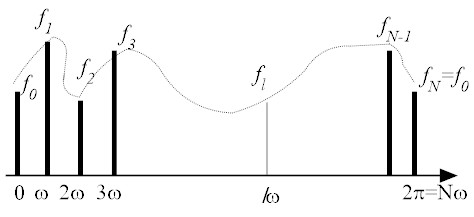
The formulas for IDFT (inverse Discrete Fourier Transform) and DFT (Discrete Fourier Transform) are
expressed as
| |
|
|
|
N−1
∑
k=0
|
Fk ei k [(2π)/(N)] l, |
| | (14) |
| |
|
|
1
N
|
|
N−1
∑
l = 0
|
fl e−i k [(2π)/(N)]l. |
| | (15) |
|
Multiply Eq. (14) by e−i m [(2 π)/(N)] l to obtain
|
fl e−i m [(2 π)/(N)] l = |
N−1
∑
k=0
|
Fk e i k [(2 π)/(N)]l e − i m [(2 π)/(N)]l. |
| (16) |
Take summation of Eq. (16) over l to get
| |
|
N−1
∑
l = 0
|
fl e− im [(2π)/(N)] l |
|
|
|
|
N−1
∑
l = 0
|
|
N−1
∑
k=0
|
Fk e i k [(2 π)/(N)]l e − i m [(2 π)/(N)]l |
| |
| |
|
|
(interchange the order of summation) |
| |
| |
|
|
|
N−1
∑
k=0
|
Fk |
N−1
∑
l = 0
|
ei (k−m) [(2 π)/(N)] l |
| |
| |
|
|
| ⎛
⎜
⎜
⎝
|
Use |
N−1
∑
l = 0
|
ei (k−m) [(2π)/(N)]l = | ⎧
⎪
⎨
⎪
⎩
|
|
| ⎞
⎟
⎟
⎠
|
|
| |
| |
|
| | (17) |
|
Hence,
| | Fm = |
1
N
|
|
N − 1
∑
l = 0
|
fl e− i m [(2 π)/(N)] l. |
| | (18) |
|
Note that in Eq. (17), we used an identity
|
|
N−1
∑
l = 0
|
ei k [(2π)/(N)] l e−i m [(2π)/(N)] l = | ⎧
⎪
⎨
⎪
⎩
|
|
|
| (19) |
which is a discrete version of
|
| ⌠
⌡
|
π
−π
|
ei k x e−i m x d x = | ⎧
⎪
⎨
⎪
⎩
|
|
|
| (20) |
(Proof of Identity (19))
Define
|
ω ≡ ei (k−m) [(2 π)/(N)]. |
|
so that
| |
|
N−1
∑
l = 0
|
ei k [(2π)/(N)] l e−i m [(2π)/(N)] l |
|
|
| |
| |
|
| | (21) |
|
If
|
k − m = 0, ±N, ±2 N, ±3N …, |
|
ω = e0, ei [(2π)/(N)] N , ei [(2π)/(N)]2 N ... = 1 so that Eq. (21) becomes
|
|
N−1
∑
l = 0
|
ei k [(2π)/(N)] l e−i m [(2π)/(N)] l = 1 + 1 + …+1 = N. |
| (22) |
On the other hand, if
|
k − m ≠ 0, ±N, ±2 N, ±3N …, |
|
Eq. (21) becomes
| |
|
| |
| |
|
|
|
1− ei (k−m) 2 π
1−ei (k−m) [(2π)/(N)]
|
|
| |
| |
|
| | (23) |
|
Therefore, it was shown that
|
|
N−1
∑
l = 0
|
ei (k−m) [(2π)/(N)]l = | ⎧
⎪
⎨
⎪
⎩
|
|
|
| (24) |
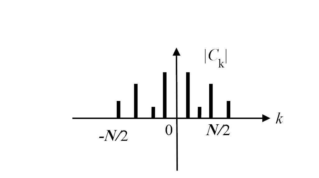
Note that only half of Fk's are independent, i.e.
The power spectrum, Pk, is symmetrical around its center, i.e.
Relation between DFT and CFT
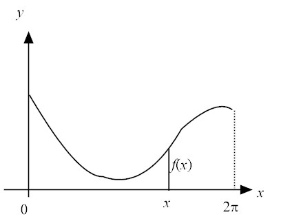
The classical Fourier series expansion of f(x) over [0, 2 π] is
| |
|
| | (27) |
| |
|
|
1
2π
|
| ⌠
⌡
|
2π
0
|
f(x) e− i k x dx. |
| | (28) |
|
If we consider an interval, 0 < x < 2 π, to be sampled at 0, [(2 π)/(N)], [(4 π)/(N)], [(6 π)/(N)] …, denoted as
|
fl ≡ f | ⎛
⎝
|
2 π
N
|
l | ⎞
⎠
|
, ω ≡ e[(2 π)/(N)]i . |
| (29) |
Then, Eq. (15) becomes
| |
|
| |
| |
|
|
|
1
N
|
|
N−1
∑
l = 0
|
| ⎛
⎝
|
∞
∑
k′=−∞
|
ck′ ωk′l | ⎞
⎠
|
ω−k l |
| |
| |
|
|
|
∞
∑
k′=−∞
|
ck′ | ⎛
⎝
|
1
N
|
|
N−1
∑
l = 0
|
ω(k′−k)l | ⎞
⎠
|
. |
| |
| |
|
|
| ⎛
⎜
⎜
⎝
|
Use |
N−1
∑
l = 0
|
ei (k−k′) [(2π)/(N)]l = | ⎧
⎪
⎨
⎪
⎩
|
|
| ⎞
⎟
⎟
⎠
|
|
| |
| |
|
|
|
∞
∑
k′=−∞
|
ck′ ×(1 if and only if k′=k, k±N, k±2N, k±3N, …, otherwise 0) |
| |
| |
|
|
ck + ck±N + ck±2 N + ck±3N +… |
| |
| |
|
| | (30) |
|
Equation (30) is the discrete version of the Nyquist sampling theorem.
If the data set does not contain components whose frequencies are higher than N/2 or |k| < N/2, DFT is identical
to CFS (classical Fourier series).
Convolution Theorem of DFT
The convolution between fl and gl is defined as
|
fl * gl ≡ |
1
N
|
|
N−1
∑
m=0
|
fl−m gm. |
| (31) |
Note that
(DFT Convolution Theorem)
|
fl * gl = |
1
N
|
|
N−1
∑
k=0
|
Fk Gk ei [(2π)/(N)] k, |
|
or DFT of fl * gl is Fk Gk.
Parseval's theorem of DFT
|
|
1
N
|
|
N−1
∑
l = 0
|
fl |
-
g
|
l
|
= |
N−1
∑
k=0
|
Fk |
-
G
|
k
|
, |
| (32) |
|
|
1
N
|
|
N−1
∑
l = 0
|
||fl||2 = |
N−1
∑
k=0
|
|| Fk||2. |
| (33) |
Power spectrum in DFT is defined as
FFT
The DFT coefficients are given by Eq. (15) and are listed here again
for reference
|
Fk = |
1
N
|
|
N−1
∑
l = 0
|
fl ω−kl k = 0, 1, 2, …, (N−1), ω ≡ e2 πi/N. |
| (35) |
For each Fk, provided that fl's and ω−k's are already
stored in computer memory,
the number of multiplications required is N and the number of
required additions is N−1 so the total number of multiplications is N2 and
the total number of additions is N (N−1). If N=1000, the total
number of multiplications is one million
and the total number of additions is 999,000, thus, requiring close to 2 million operations.
FFT (Fast Fourier Transform) is an algorithm to efficiently compute the DFT coefficients which
can reduce the number of operations from N2 (multiplications) to N log2 N.
This reduction is dramatic as shown in the table below:
| N | N2 | N log2 N | Ratio |
| 10 | 100 | 33 | 3 |
| 100 | 10000 | 664 | 15 |
| 1000 | 1,000,000 | 9,900 | 100 |
| 10000 | 100 million | 0.13 million | 750 |
| 1 million | 1 trillion | 20 million | 50,100
|
Given f0, f1, f2, …fN−1, define
|
g(x) ≡ f0 + f1 x + f2 x2 + …+ fN−1 xN−1. |
| (36) |
By comparing Eq. (36) with Eq. (35), it can be readily seen that
the coefficient, Fk, can be computed by
To illustrate the algorithm of FFT, let N=8, then,
| |
|
|
f0 + f1 x + f2 x2 + f3 x3 + f4 x4 + f5 x5 + f6 x6 + f7 x7 |
| |
| |
|
|
(f0 + f2 x2 + f4 x4 + f6 x6) +x ( f1 + f3 x2 + f5 x4+ f7 x6) |
| |
| |
|
| | (38) |
|
where
|
| ⎧
⎪
⎨
⎪
⎩
|
|
p(x) ≡ f0 + f2 x + f4 x2 + f6 x3 |
|
|
q(x) ≡ f1 + f3 x + f5 x2 + f7 x3. |
|
|
|
| (39) |
Thus, to compute all the coefficients of Fk is equivalent to
computing both p(x2) and q(x2) at
x=1, ω, ω2, ω3, ω4, ω5, ω6, ω7, multiplying
x by q(x2) and add them together.
It should be noted that for
|
x=1, ω, ω2, ω3, ω4, ω5, ω6, ω7, |
| (40) |
the corresponding x2's are (note ω8=1)
| |
|
|
1, ω2, ω4, ω6, ω8, ω10, ω12, ω14 |
| |
| |
|
| 1, ω2, ω4, ω6, 1, ω2, ω4, ω6. |
| | (41) |
|
It is seen that the second half of x2 are the repetition of
the first half, thus, it is NOT necessary
to compute p(x2) and q(x2) when x belongs to the second half.
Moreover, note that the set of {1, ω2, ω4, ω6} is
the roots to
so computing p(x2) and q(x2) is equivalent to
computing p(x) and q(x) where x is the root for x4=1 (a half of the order 8).
Therefore, if the number of multiplications to compute FFT of the N-th order is denoted as
M(N), it must satisfy
where the factor "2" comes from the computation of p(x2) and q(x2),
the argument, N/2, of M comes from the equation of x4 = 1 (x(N/2)=1) and
the last term of N is for the multiplication between x and q(x2) for N times.
When N=1, g(x)=f0, thus,
From Eqs.(43-44), the solution to Eq. (43) is
Similarly, the number of additions can be computed as
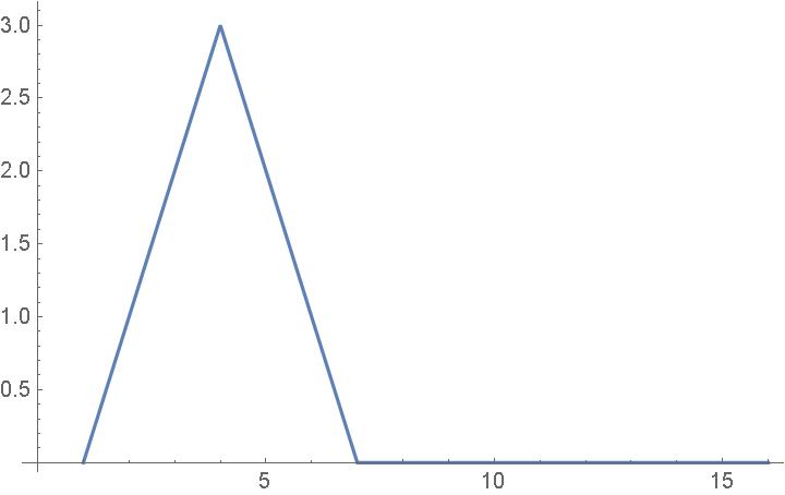
Example 1
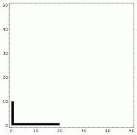
Consider a data set of (N=16)
|
f1 = {0, 1, 2, 3, 2, 1, 0, 0, 0, 0, 0, 0, 0, 0, 0, 0 } |
| (47) |
which looks like
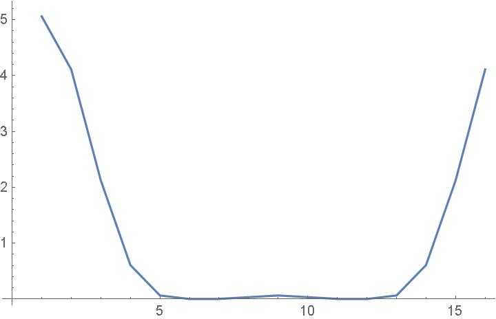
The power spectrum, |Ck|2, of f1 is
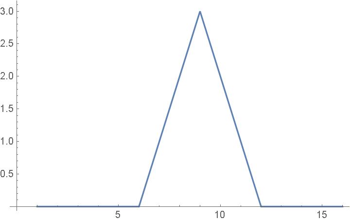
Now consider
|
f2={0, 0, 0, 0, 0, 0, 1, 2, 3, 2, 1, 0, 0, 0, 0, 0} |
| (48) |
The power spectrum, |Ck|2, of f2 is
Example 2 (2-D)
Consider two different images
 , ,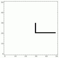 |
The power spectra of the images
are shown as
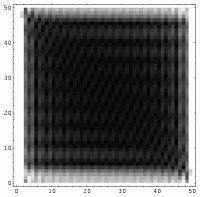 , , |
They are identical each other even though
the spatial representations are different.
It can be indeed shown that the correlation between the two graphs of the power spectra is 100%.
Example 3
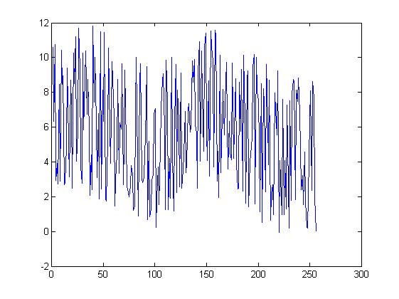 Using the fft (Fast Fourier Transform) and ifft
(Inverse Fourier Transform)
functions available in MATLAB/
OCTAVE, remove the noise from the data above and restore the original signal.
You can copy and paste the following line to enter the data into MATLAB/OCTAVE.
Using the fft (Fast Fourier Transform) and ifft
(Inverse Fourier Transform)
functions available in MATLAB/
OCTAVE, remove the noise from the data above and restore the original signal.
You can copy and paste the following line to enter the data into MATLAB/OCTAVE.
y=[10.5998892219547 6.32715963943755 10.7418564397819 2.9411380441864 3.92528722303704 2.71618105372149 8.4617982675031 2.88080944171953 10.4141369874892 8.476032583145489 8.964925641878001 2.67576180217924 2.85081602904105 4.85231952204638 9.38358373297042 5.16481823892903 3.14070937711815 8.699875412947099 7.21927535505636 2.47218681863012 10.2726165797325 8.500254531789301 11.1978723384108 4.05021576256659 5.77322285188005 11.7074336020358 9.400871264109419 3.71878673302725 2.78562995675663 10.2401630961987 5.84306139392084 8.82789975382806 10.3993315932854 6.74306607935596 8.750462753122729 5.90480261238712 2.06109189130585 4.40535088299872 2.41192556568313 11.8214297012451 7.44250415683415 10.032769833142 6.28901765997294 3.08186615850219 6.76595055198963 1.87944040723309 11.502034897292 2.44379054233261 8.128891862212489 6.34299932572315 11.4665531337537 1.86621678597553 1.75517155481136 5.19324241215718 10.5420445171336 5.82311606131353 3.92802666444074 9.77260830545065 8.76106471812958 6.54554696769744 1.4624210554122 2.92068844004011 4.48263396519447 8.739554957492571 3.33478186865148 6.24348148116228 5.87860301757644 9.666406406463951 2.70299316464037 5.01601721808914 9.26536386544738 5.09532896085959 2.62513156468079 2.21732831519875 1.99448077033047 2.62844514632015 3.79686487481322 3.24327464459272 1.2326443145944 1.45988948327978 7.1131310391548 10.0220774080567 3.93470053413877 0.894329071535874 8.60989560717546 9.63540704314247 3.00857673282652 2.79007156060591 3.15054286446995 4.53048193808516 5.38399703002467 9.4833604924008 0.6953758598942 5.19383112351193 0.844822890049153 1.34649332130299 2.98525367766063 3.31627989414972 6.76285368200212 7.04875327912278 0.251045988826941 1.9108517787023 3.69941930619919 1.52517099472442 4.831074892421 7.11794613059188 8.72763093617244 9.078887558695371 5.89633680306463 1.24117091269616 9.850706571849731 7.44945101897683 1.24091019808261 4.18876971107157 1.9176033724533 9.995859008983791 4.06138975672046 1.15781821760705 6.39682907701427 9.58794591991612 2.2193562129817 8.15089615664534 6.25502635127747 2.54857914360014 9.129606203212679 2.4736245862179 3.56168512084511 4.43958848222138 6.8931750450365 3.37222234736257 3.90894160047792 7.00239599243425 7.36043668237722 5.72237545873726 6.02879296664729 9.802065832144031 8.575987244312429 9.897577054258401 6.18523789886617 5.69121169822893 2.46963366954875 9.129229771930889 10.8952016844065 4.04009660589757 10.3743854729916 7.86000365182057 4.62415698798384 10.6214785584302 11.4224951621026 5.67326994393055 4.08637580957679 8.65738342494789 3.19239876321067 11.5201022637337 10.636312915602 9.82811239395342 3.70890071720701 11.5798531399931 11.3079723127561 2.91023922097878 4.62563348751362 1.94134261430337 10.1199743509774 3.39739911000981 6.74500334449411 8.170425024996179 5.56015657871609 7.5183998639944 9.724435694474771 6.0923080693899 3.59482558370596 6.31863247939307 4.52463371931999 4.10296747447814 9.695171467636451 4.18461466022538 5.80815539286633 8.77375948273572 3.89726672007424 2.4379111867341 2.53028144217005 8.599734675735849 5.73721564890586 9.31292716873403 2.30164223598104 10.1205267404267 6.46257375724972 1.61357790565941 8.83703123702375 9.241195975932539 1.39848359552096 4.04514624784499 4.45713558113789 5.40256645503303 9.458465543021051 10.1594053991668 1.57320417124056 10.025068241083 8.050843440082611 7.57425636264847 4.99279654689739 1.14890755632154 8.48815583223322 0.513616604704808 8.20951495224771 7.36944262027792 2.28314474381409 9.61805543347821 6.38395393390104 3.82496380452266 8.716233740636451 0.624777553892277 2.13639412542771 2.67182229714328 0.960693039360867 7.94782117163402 6.97092617961824 5.54658352916538 9.25358919832107 -0.0518943288602689 4.09372366108078 3.0771241498034 0.9687056105548451 7.58002335011327 0.964153518012499 4.05886921736417 1.30771587473559 7.28546269899251 2.60725514587506 0.181148813423656 7.50124107556926 1.78225486901118 7.93044999804643 8.726414919885549 8.64856640820909 1.81661636398602 8.15011697120986 7.48520651711012 8.821324599765621 6.77111885101838 4.83400122253399 2.39038025124365 3.22625506903038 1.55735245264944 4.56184163155081 1.75825250678772 0.269608991651202 0.197345665382678 4.06499325144136 6.52779016528276 8.09415174197148 2.37792649587988 8.6329654872403 7.66695265328003 1.99742029842287 0.0182366166899817];
This variable, y, contains 256 data points.
Adjust the default directory, i.e.
Method 1
cd c:/tmp
% CD to the "c:/tmp" directory
%
y=[...............];
%
plot(y);
f1=fft(y); % Fast Fourier Transform of y, i.e. frequency domain expression of y
plot(abs(f1)); % Since f1 is a set of complex numbers, we take only the absolute values.
%
% Examine the graph of f1 (in frequency) and determine the cut-off values.
%
% Filtering out data with small amplitude
%
for i=1:256
 if abs(f1(i)) < 50
   f1(i)=0;
 end;
end;
%
% (alternative way)
% f1(abs(f1)<50)=0;
%
% Inverse FFT on f1
%
y2=ifft(f1);
%
% y2 is real but there is some dust so chop them off.
%
y2=real(y2);
plot(y2);
|
Method 2
cd c:/tmp
% CD to the "c:/tmp" directory
%
y=[...............];
%
plot(y);
f1=fft(y);
plot(abs(f1));
%
% define filter
%
fil=zeros(1, 256);
fil(1, 1:3)=1;
fil(1,253:256)=1;
%
f2=fil.*f1;
%
plot(abs(f2));
y2=ifft(f2);
plot(real(y2));
|
Example 4
Wave file
cd c:\tmp
x=audioread('cricket.wav');
[n, m]=size(x)

y=fft(x);
y2=abs(y);
plot(y2);
semilogx(y2);
% around 10^5
%
fil=zeros(n,m);
w1=40000;w2=100000;
fil(w1:w2, :)=1;
fil(n-w2:n-w1, :)=1;
%
y3=fil.*y;
x2=ifft(y3);
%
fs=44100;
%
audiowrite('cricket2.wav', real(x2), fs);
Note: Use wavread and wavwrite in Octave instead of audioread and audiowrite. Use wavwrite(ifft(y), 44100, 'newwavefile.wav');
Filtered wave file
Definition of DFT
- Our definition
| |
|
|
|
N−1
∑
k=0
|
Fk ei k [(2π)/(N)]l |
| | (49) |
| |
|
|
1
N
|
|
N−1
∑
k=0
|
fl e−i k [(2π)/(N)]l |
| | (50) |
|
- MATLAB/Octave
| |
|
|
|
1
N
|
|
N−1
∑
k=0
|
Fk ei k [(2π)/(N)]l |
| | (51) |
| |
|
|
N−1
∑
k=0
|
fl e−i k [(2π)/(N)]l |
| | (52) |
|
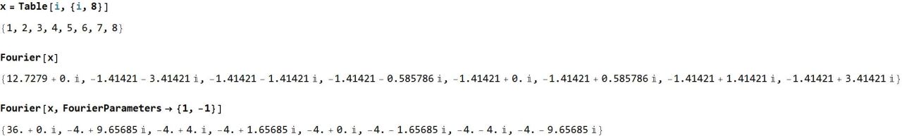
- Mathematica
| |
|
|
|
1
√N
|
|
N−1
∑
k=0
|
Fk e−i k [(2π)/(N)]l |
| | (53) |
| |
|
|
1
√N
|
|
N−1
∑
k=0
|
fl ei k [(2π)/(N)]l |
| | (54) |
|
octave.exe:1> x=1:8
x =

   1   2   3   4   5   6   7   8

octave.exe:2> fft(x)
ans =

 Columns 1 through 4:

   36.0000 +  0.0000i   -4.0000 +  9.6569i   -4.0000 +  4.0000i   -4.0000 +  1.6569i

 Columns 5 through 8:

   -4.0000 +  0.0000i   -4.0000 -  1.6569i   -4.0000 -  4.0000i   -4.0000 -  9.6569i
Footnotes:
1
where ω is an angular frequency (unit: rad/time) and f is a (regular) frequency (unit: Hz).
2
|
f(x)= |
∞
∑
m=−∞
|
cm ei mx, cm = |
1
2π
|
| ⌠
⌡
|
2π
0
|
f(x)e−imx dx. |
|
3
A more aggressive algorithm yields
which results in
|
M(N) = |
N
2
|
log2 N − |
3
2
|
N + 2. |
|
File translated from
TEX
by
TTH,
version 4.03.
On 03 Nov 2025, 22:45.