| (1) |
| (2) |
| (3) |
|
|
|
|
|
 |
|
|
 |
|
|
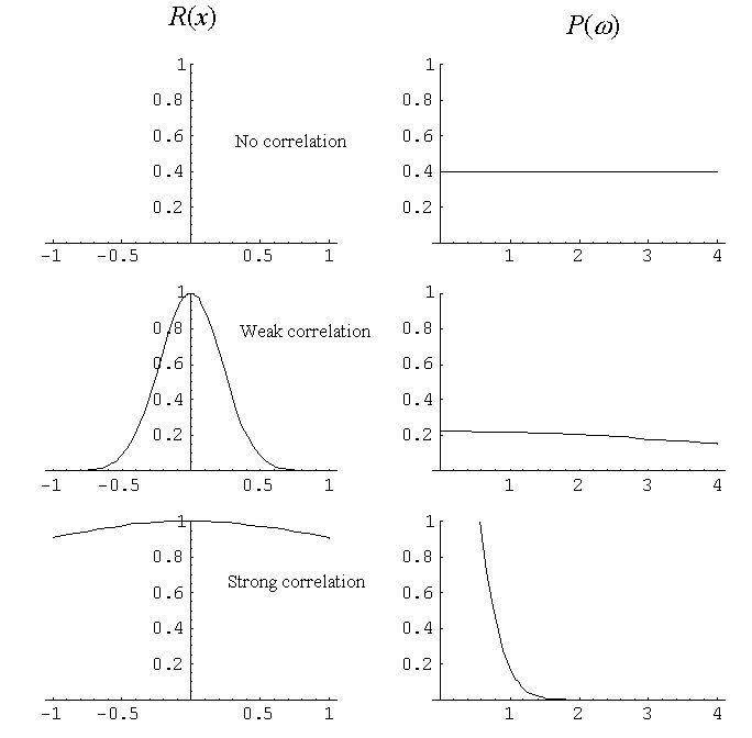 If P(ω) is independent of the frequency, it is called white noise.
If P(ω) is approximately proportional to 1/f ( = 1/ω), the original data is called pink noise,
1/f noise or fractal noise and if P(ω) is approximately proportional to 1/f2, it is called
brownian (red) noise.
If P(ω) is independent of the frequency, it is called white noise.
If P(ω) is approximately proportional to 1/f ( = 1/ω), the original data is called pink noise,
1/f noise or fractal noise and if P(ω) is approximately proportional to 1/f2, it is called
brownian (red) noise.
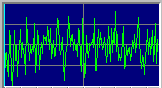 White noise
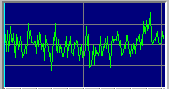 Pink noise
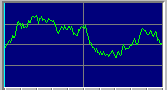 Brownian (red) noise
Another site
| (5) |
| (6) |
| (7) |
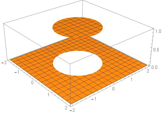
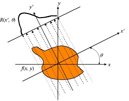 Note that R(x′, θ) depends on x′ and θ.
The Fourier transform for a two variable function, f(x, y), is defined as
Note that R(x′, θ) depends on x′ and θ.
The Fourier transform for a two variable function, f(x, y), is defined as
| (8) |
| (9) |
| (10) |
|
| (12) |
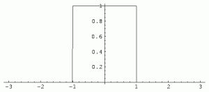
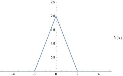
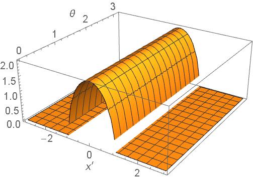
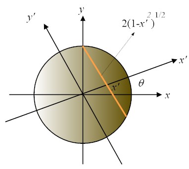 The Radon transform of the function,
| (13) |
| (14) |
|
|