


| (1) |
| (2) |
|
| (3) |
| (4) |
|
| (6) |
|
| (10) |
| (11) |
| (12) |
|
| (13) |
| (14) |
|
|
|
|
|
| (21) |
| (22) |
| (23) |
| (24) |
|
| (26) |
| (27) |
| (28) |
| (29) |
| (30) |
| (31) |
| (32) |
 |
 |
|
|
| (37) |
| (38) |
 |
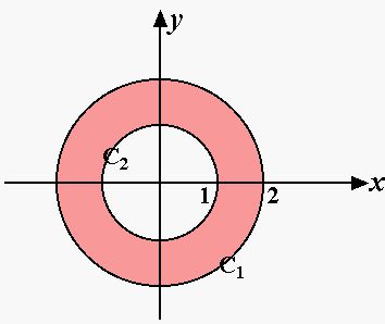 Note that along C1, v=(x, y) = (2 cos θ, 2sin θ),
and along C2, v=(x, y)=( cos θ, sin θ).
Note that along C1, v=(x, y) = (2 cos θ, 2sin θ),
and along C2, v=(x, y)=( cos θ, sin θ).
|
|
|
|
| (46) |
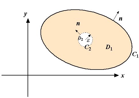 When the above identity is applied to a multiply-connected body with a circular hole
centered at x with the radius, ϵ,
Eq.(46) becomes
When the above identity is applied to a multiply-connected body with a circular hole
centered at x with the radius, ϵ,
Eq.(46) becomes
| (47) |
| (48) |
| (49) |
| (50) |
| (51) |
| (52) |
| (53) |
|
|
| (58) |
| (59) |
| (60) |
|
|
|
|
|