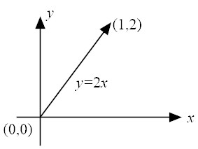
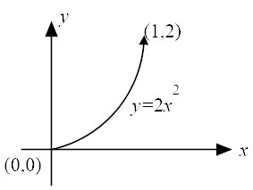
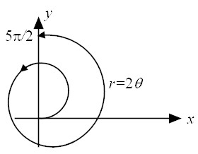
While the line integrals of Examples 1 and 2 depend on the integral
path, the line integral of Example 3 is independent of the path.
This difference will be clarified in the next section.
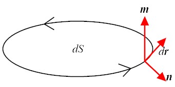
Stokes' theorem
⌠ (⎜) ⌡
∂S
F·dr =
⌠ ⌡
⌠ ⌡
S
m·(∇×F)dS.
(10)
Proof
From the figure above,
dr = m×ndr,
so it follows that
⌠ (⎜) ⌡
∂S
F ·dr
=
⌠ (⎜) ⌡
∂S
F ·(m ×n) dr
=
(scalartripleproduct)
=
⌠ (⎜) ⌡
∂S
m ·(n ×F) dr
=
(Gausstheorem)
=
⌠ ⌡
⌠ ⌡
S
m ·(∇×F) dS.
(11)
Example
The velocity field of a vortex that rotates with the angular velocity of ω is given as
v
=
r ωeθ
=
r ω
⎛ ⎜ ⎜
⎜ ⎝
−sinθ
cosθ
0
⎞ ⎟ ⎟
⎟ ⎠
=
⎛ ⎜ ⎜
⎜ ⎝
−ωy
ωx
0
⎞ ⎟ ⎟
⎟ ⎠
,
(12)
so
∇×v = 2 ωk.
(13)
If F=(P, Q, 0), m=(0,0,1) and the Stokes' theorem is rewritten
as
⌠ (⎜) ⌡
∂S
Pdx + Qdy =
⌠ ⌡
⌠ ⌡
S
⎛ ⎝
∂Q
∂x
−
∂P
∂y
⎞ ⎠
dA.
(14)
Irrotational Field
Definition: If the vector field, v, satisfies
∇×v=0, v is called an irrotational field.
Theorem: The following four statements are all equivalent.
(1)


 Proof
From the figure above,
Proof
From the figure above,