


#10 (09/22/2025)
Divergence theorem (Gauss theorem)
Remember the definition of the divergence operator for 2-D as
where n is the normal to the boundary, ∆s is the surface area of
the object, and ∂S is the boundary of the
object domain. This definition has an advantage over other definitions as it
is independent of the coordinate system.
Equation (1) is approximately written as
|
| ⌠
(⎜)
⌡
|
∂S
|
n·u dl ∼ ∇·u ∆s. |
| (2) |
If Eq.(2) is applied to the two regions below,
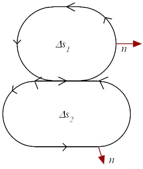 it follows
which can be added together to yield
|
| ⌠
(⎜)
⌡
|
∂(s1 + s2)
|
n·u dl ∼ | ⌠
⌡
|
| ⌠
⌡
|
∇·u dS. |
| (5) |
By repeating this for many small cells and
taking limit of ∆si → 0,
Eq.(5) becomes
|
| ⌠
(⎜)
⌡
|
∂S
|
n ·u dl = | ⌠
⌡
|
| ⌠
⌡
|
S
|
∇·u dS. |
| (6) |
This is called the Gauss divergence theorem.
Verification
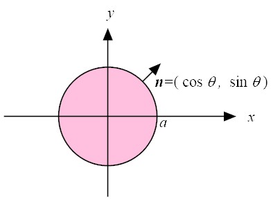
(LHS)
On the boundary, one can set
and
On the boundary, one can set
so
|
n·u = a3 cos3 θsin θ+a sinθ(cos θ+sin θ), |
| (11) |
and
| |
|
|
| ⌠
⌡
|
2π
0
|
( a3 cos3 θsin θ+a sinθ(cos θ+ sin θ) )a dθ |
| |
| |
|
| | (12) |
|
(RHS)
Use the polar coordinate system, i.e.
|
x = r cosθ, y = r sin θ, dS = r dr dθ. |
|
As
so
| |
|
|
| ⌠
⌡
|
| ⌠
⌡
|
S
|
(2 x y + 1) dx dy |
| |
| |
|
|
| ⌠
⌡
|
2π
0
|
| ⌠
⌡
|
a
0
|
(2 r2 cos θsin θ+1) r dr dθ |
| |
| |
|
| | (14) |
|
Alternative interpretation of Gauss theorem
 The fundamental theorem of calculus postulates that integrations and
differentiations are reciprocal to each other, i.e.
The fundamental theorem of calculus postulates that integrations and
differentiations are reciprocal to each other, i.e.
|
| ⌠
⌡
|
b
a
|
f ′(x) dx = [ f ]ab. |
| (15) |
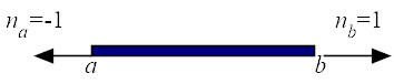
The right hand side of Eq.(15) can be written as
| |
|
| |
| |
|
|
(−1) ×f |x=a + (+1) ×f |x=b |
| |
| |
|
|
na f |x = a + nb f |x = b |
| |
| |
|
| |
| |
|
| | (16) |
|
So Eq.(15) can be written as
|
| ⌠
⌡
|
b
a
|
f ′(x) dx = |
∑
boundary
|
n f. |
| (17) |
Equation (17) can be extended to 2-D as
|
| ⌠
⌡
|
| ⌠
⌡
|
S
|
∇f dS = | ⌠
(⎜)
⌡
|
∂S
|
n f dl. |
| (18) |
Note that both ∇ and n are vectors.
If we set f = u (vector), Eq.(18) can be written as
|
| ⌠
⌡
|
| ⌠
⌡
|
S
|
∇·u dS = | ⌠
(⎜)
⌡
|
∂S
|
n ·u dl, |
| (19) |
which is the Gauss divergence theorem.
Note that most of the usage of the divergence theorem is to convert a boundary integral
that contains the normal
to the boundary into a volume (area) integral
by replacing the normal (n) by a nabla (∇) to be placed in front of the
expression.
|
| ⌠
(⎜)
⌡
|
∂S
|
…n …dl = | ⌠
⌡
|
| ⌠
⌡
|
S
|
∇…dS. |
| (20) |
Integration by parts
Integrating the both sides of
yields
|
| ⌠
⌡
|
b
a
|
( u v ) ′d x = | ⌠
⌡
|
b
a
|
u ′v dx + | ⌠
⌡
|
b
a
|
u v ′dx, |
| (22) |
or
|
[ u v ]ab = | ⌠
⌡
|
b
a
|
u ′v dx + | ⌠
⌡
|
b
a
|
u v ′dx, |
| (23) |
or
|
| ⌠
⌡
|
b
a
|
u′v dx = [ uv]ab − | ⌠
⌡
|
b
a
|
uv′dx. |
| (24) |
Equation (24) is the 1-D formula for integration by parts.
Equation (24) can be extended to 2D as
|
| ⌠
⌡
|
| ⌠
⌡
|
S
|
∇u v dS = | ⌠
(⎜)
⌡
|
∂S
|
u v n dl− | ⌠
⌡
|
| ⌠
⌡
|
S
|
u ∇v dS. |
| (25) |
Example
(Green's identity)
|
| ⌠
⌡
|
| ⌠
⌡
|
S
|
(∇u ·∇v + u ∆v) dS = | ⌠
(⎜)
⌡
|
∂S
|
u |
∂v
∂n
|
dl. |
| (26) |
Proof:
Rewrite the right hand side of Eq.(26) as
which is a boundary integral with n.
Therefore, according to the Gauss theorem, it follows
| |
|
| |
| |
|
|
| ⌠
⌡
|
| ⌠
⌡
|
S
|
( ∇u ·∇v + u ∇·∇v) d S |
| |
| |
|
| ⌠
⌡
|
| ⌠
⌡
|
S
|
( ∇u ·∇v + u ∆v) d S . |
| | (28) |
|
Examples
- Heat conduction
The balance of energy is stated as
|
| ⌠
⌡
|
| ⌠
⌡
|
S
|
ρCp |
∂T
∂t
|
dS = | ⌠
(⎜)
⌡
|
∂S
|
(−n) ·h dl, |
| (29) |
where ρ is the mass density, Cp is the specific heat, h is the heat flux across
the boundary of the control surface.
Using the Gauss theorem, the right hand side of Eq.(29)
becomes
|
| ⌠
(⎜)
⌡
|
∂S
|
(−n) ·h dl = − | ⌠
⌡
|
| ⌠
⌡
|
S
|
∇·h dS, |
| (30) |
so it follows
|
| ⌠
⌡
|
| ⌠
⌡
|
S
|
ρCp |
∂T
∂t
|
dS = − | ⌠
⌡
|
| ⌠
⌡
|
S
|
∇·h dS, |
| (31) |
or
Using Fourier's law,
where k is the thermal conductivity, Eq.(32) becomes
- Equilibrium equation in static elasticity
The balance of force for continua is stated as
|
| ⌠
(⎜)
⌡
|
∂S
|
t dl+ | ⌠
⌡
|
| ⌠
⌡
|
S
|
b dS=0, |
| (35) |
where t is the surface traction force and b is the body force.
The surface traction force t is the contribution of the stress tensor,
σ, in the direction of n as
so Eq.(35) becomes
|
| ⌠
(⎜)
⌡
|
∂S
|
σ·n dl+ | ⌠
⌡
|
| ⌠
⌡
|
S
|
b dS=0, |
| (37) |
or
|
| ⌠
⌡
|
| ⌠
⌡
|
S
|
∇·σdS + | ⌠
⌡
|
| ⌠
⌡
|
S
|
b dS=0, |
| (38) |
or
which is known as the equation of equilibrium. For small elastic deformation,
where C is the elastic modulus and u is the displacement, Eq.(39) becomes
which is known as the Navier's equation
2.
- Green's second identity
|
| ⌠
⌡
|
| ⌠
⌡
|
S
|
(u ∆v − v ∆u) dS = | ⌠
(⎜)
⌡
|
∂S
|
| ⎛
⎝
|
u |
∂v
∂n
|
− v |
∂u
∂n
| ⎞
⎠
|
dl. |
|
From the first Green's identity,
Subtracting Eq.(43) from Eq.(42) gives the second
Green's identity. This identity is used to derive solutions to
Poisson's equation (∆u = −ρ).
Footnotes:
1
Enter a^4 Cos[x]^3 Sin[x] +a^2 Sin[x]Cos[x]+a^2 Sin[x]^2, x, 0, 2 Pi
(you can copy and paste with the mouse.)
2
Each quantity is a tensor.
File translated from
TEX
by
TTH,
version 4.03.
On 21 Sep 2025, 13:52.