


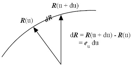
 The length of a curved line from u = u to u = u + du can be
computed by carrying out integration of ds (line segment)
The length of a curved line from u = u to u = u + du can be
computed by carrying out integration of ds (line segment)
|
|
|
| (3) |
 Solution
As
Solution
As
|
|
|
|
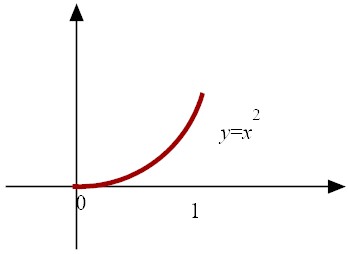
Sqrt[1 + 4 u^2] u 0 1exactly (case sensitive, square bracket) in the boxes then press the query button.

|
 |
|
|
|
|
|
| (9) |
|
| (12) |
| (13) |
| (14) |
 |
| (15) |
| (16) |
|
|
|
| (25) |
| (26) |
| (27) |
| (28) |
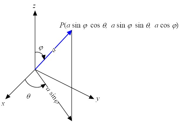
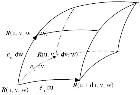 The volume element of the parallelepiped spanned by the three vectors above
can be expressed as3
The volume element of the parallelepiped spanned by the three vectors above
can be expressed as3
| (29) |
 |
| (30) |
| (31) |
| (32) |
| (33) |
|
|
|
|
| (35) |
 |
|
 |
| (39) |
| (40) |
| (41) |
| (42) |
| (43) |
|
| (46) |
| (47) |
| (48) |
| (49) |
| (50) |
| (51) |
| (52) |
| (53) |
|
|
| (56) |
| (57) |
| (58) |
|
|