#07 (09/10/2025)
Implicit functions
If the relationship between x and y is given implicitly as
it is still possible to express y as a function of x by Taylor series
about x = a as
|
y(x) = y(a) + y′(a)(x − a) + |
y"(a)
2!
|
(x − a)2 + |
y"′(a)
3!
|
(x − a)3 + … |
| (2) |
if y(a), y′(a), y"(a) … are known. One can differentiate
f(x, y) = 0 with respect to x to get y′(x) without explicitly
solving f(x, y) = 0 for y(x) as
|
fx (x, y) + fy(x, y) y′(x) = 0, |
| (3) |
or
|
y′(x) = − |
fx(x,y)
fy(x,y)
|
. |
| (4) |
Once y′(x) is obtained, y"(x) can be derived by differentiating
the both sides of y′(x) with respect to x again
1 as
| |
|
|
− |
(fxx + fxy y′)fy − fx (fyx + fyyy′)
fy2
|
|
| |
| |
|
|
− |
|
| ⎛
⎝
|
fxx + fxy ( |
− fx
fy
|
) | ⎞
⎠
|
fy − fx | ⎛
⎝
|
fyx + fyy( |
− fx
fy
|
) | ⎞
⎠
|
fy2
|
|
| |
| |
|
|
2fx fy fxy −fx2 fyy − fy2 fxx
fy3
|
, |
| | (5) |
|
and other higher order derivatives can be obtained in a similar manner.
It is seen that for y = y(x) to exist at x = x0,
the denominator of fy must not vanish, i.e.
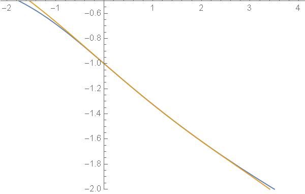
Example
Expand y(x) about x = 1 up to and including second
order for
|
f(x, y) ≡ x y −y3 − 1 = 0. |
| (7) |
Solution: The Taylor series of y(x) about x=1 is
|
y(x) = y(1) + y′(1)(x − 1) + y"(1)/2! (x − 1)2 + … |
| (8) |
By substituting
x = 1 into x y − y3 − 1 = 0, one gets y(1) = −1.32 … by solving
y − y3 − 1 = 0 (there are two other complex roots but are not considered
here). Next, by differentiation x y − y3 − 1 = 0 with respect to x (note
that y is a function of x), one gets
y + x y′− 3 y2 y′ = 0 which can be solved for y′ as
y′ = y/(3 y2 − x). This can be further differentiated with respect to x
as y" = (y′(3y2 − x) − y(6 y y′−1))/(3 y2 − x)2 so it is possible to
obtain y(1), y′(1), y"(1), ... sequentially.
Finally, one obtains
|
y(x) = −1.32472 −0.310629 (x−1) +0.0170796 (x−1)2+0.00114503 (x−1)3 −0.00128188 (x−1)4+ … |
| (9) |
Application:Lagrange multiplier
As an application of the theory of implicit functions, the Lagrange
multiplier method is discussed here.
We want to extremize f(x, y)
subject to the constraint, g(x, y) = 0.
Assuming g(x, y) = 0 can be
solved for y as y = y(x), this is substituted into the object
function of f(x, y) as f(x, y(x)) thus we can look at f(x, y(x)) as
a function of x.
The candidates of x's to extremize f can be
obtained by differentiating f with respect to x as
where y′ in Eq.(10) can be obtained from g(x, y) = 0 as
Substituting Eq.(11) to Eq.(10) yields
where λ is a newly introduced parameter called the Lagrange multiplier.
The development above implies that when extremizing f(x, y)
subject to g(x, y) = 0, instead of working on f(x, y), one can
try extremizing
without any constraint, i.e. partially differentiating
Eq.(13) with respect to x, y and λ
as
The above equations form a set of simultaneous equations for x, y and λ.
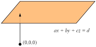
Example 1
Find the shortest distance from the origin (0, 0, 0)
to the plane, a x + b y + c z = d.
|
f(x, y, z) = x2 + y2 + z2 → min |
| (17) |
|
subject to g(x, y, z) = a x + b y + c z − d = 0. |
| (18) |
Instead of minimizing f(x, y, z) with the constraint, one can try
minimizing f*(x, y, z) ≡ f(x, y, z) − λg(x, y, z)
with respect to x, y, z and λ without any
constraint.
Solving the above set of simultaneous equations yields
or equivalently
so the minimum distance is
Alternative approach: Read the problem as
Find the shortest distance from the origin (0, 0, 0)
to the plane, a x + b y + c z = d.
 The plane, a x + b y + c z = d, is also expressed as
where a = (a, b, c) and x = (x, y, z). Equation (31) implies that
the vector a is perpendicular to the plane (as was shown in class). Hence, the
vector from the origin that minimizes the distance to the plane must be expressed as
where t is a parameter. By substituting Eq.(32) into Eq.(31), one obtains
Hence, t can be solved as
From Eq.(32), it follows
and the length of x is
Example 2
Find the shortest distance from (1, 0) to x3 − 2 y2 = 0.
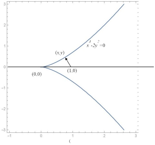 (Solution)
Let
(Solution)
Let
|
f* ≡ (x −1)2 + y2 − λ(x3 − 2 y2), |
|
it follows
The above equations can be solved as (real roots)
|
(x, y, λ) = ( |
2
3
|
, |
2
3 √3
|
, − |
1
2
|
) or ( |
2
3
|
, − |
2
3 √3
|
, − |
1
2
|
), |
| (40) |
both of which yield
|
d = |
√
|
(x−1)2 + y2
|
= |
⎛
√
|
|
∼ 0.509175. |
| (41) |
Sample MATLAB/Octave code:
x=1; y=1; lambda=1;

for i=0:10
 eqs=[ 2*(x-1)-3*x*x*lambda ; 2*y+4 *y *lambda ; -x^3+2*y*y];

 jacob=[2-6*x*lambda, 0, -3*x*x; 0, 2+4*lambda, 4*y; -3*x*x, 4*y, 0];

 right=inv(jacob)*eqs;

 x=x-right(1);
 y=y-right(2);
 lambda=lambda-right(3);
end;

fprintf('%f %f %f\n', x, y,lambda);
fprintf('%f', sqrt((x-1)^2+y^2));
Online C compiler
Online MATLAB/Octave
Wolfram Alpha
Vector Analysis
Scalar product (inner product, dot product)
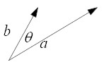
The scalar product between the two vectors, a and
b, is defined as
where θ is the angle between the two vectors.
 The following properties can be derived based on the
definition of Eq.(42).
The following properties can be derived based on the
definition of Eq.(42).
- a ·b = b ·a
- c a ·b = a ·c b = c (a ·b)
- a ·(b + c ) = a ·b + a ·c
It is possible to derive the scalar product in terms of the components
of a vector by introducing the base vectors, ex and ey. Note that
Using Eq.(43), the scalar product of two vectors
in components is
| |
|
|
(ax ex +ay ey )·(bx ex +by ey ) |
| |
| |
|
|
ax bx ex ·ex + ax by ex ·ey + ay bx ey ·ex + ay by ey ·ey |
| |
| |
|
| | (44) |
|
The definition of Eq.(42) is a preferred form as it is
independent of the coordinate system.
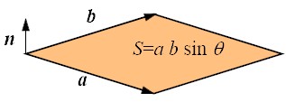
Vector product (cross product)
The vector product is defined between two vectors in 3-D as
where S is the area of the parallelogram spanned by the two vectors and
n is the unit vector whose direction is in the right hand
system as shown in the figure.
The following properties can be derived based on the
definition of Eq.(45).
- a ×b = −b ×a
- c a ×b = a ×c b = c (a ×b)
- a ×(b + c ) = a ×b + a ×c
Note that a×a = 0 (no area by two identical
vectors).
The relationship among 3-D base vectors is summarized as
and
|
ex ×ex = ey ×ey = ez ×ez = 0. |
| (47) |
Using the relationship above, the vector product is expressed
in components as
| |
|
|
(ax ex +ay ey +az ez )×(bx ex +by ey +bz ez ) |
| |
| |
|
|
ax bx ex×ex+ax by ex×ey+ax bz ex×ez+ … |
| |
| |
|
| |
| |
|
| | (48) |
|
Equation of plane (application of dot product)
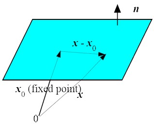 The relationship among x0 (fixed point),
x (moving point) and n (normal, fixed vector) is
The relationship among x0 (fixed point),
x (moving point) and n (normal, fixed vector) is
So the equation of a plane is expressed as
Note that c represents the shortest distance between the plane
and the origin.
Triple products
There are two types of vector products, scalar triple product and
vector triple product, whose main usage is found in vector analysis.
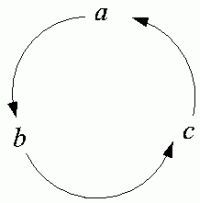
Scalar triple products, a·(b×c)
a·(b×c) = a·S n = S a cosθ = S h represents the volume of the parallelepiped
spanned by the three vectors, a, b and c.
Note the cyclic relationship below.
a·(b×c) = b·(c×a) = c·(a×b)
Vector triple products, a ×(b×c)
|
a ×(b×c) = (a·c)b − (a·b)c. |
|
Note that the right hand side is a combination of
b and c both of which are inside the parentheses in the
left hand side. The one that is in the middle (b) comes first.
Exercise
- a×( b×c) +b×( c×a) +c×( a×b) = ?
-
(a×b)·(c×d) = ?
Footnotes:
1
|
| ⎛
⎝
|
u
v
| ⎞
⎠
|
′
|
= |
u′v − u v′
v2
|
. |
|
File translated from
TEX
by
TTH,
version 4.03.
On 09 Sep 2025, 23:05.