#05 (09/03/2025)

Another example of error analysis in numerical integration

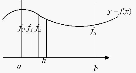
The (left) rectangular rule is expressed as

R_n = h ( f₀ + f₁ + f₂ + f₃ + …+ f_n−1).

It was shown that

I ∼ R_n + A h.

(1)

By halving the step size, one gets

I ∼ R_{2 n} + A

(2)

Subtracting Eq.(1) from twice Eq(2), one obtains

I ∼ 2 R_{2 n} − R_n,

(3)

which eliminates the error in the order of h. Note that if h is the step size for 2 n partitions, the step size for n partitions is 2 h.

Hence,

∼

2 R_{2 n} − R_n

2 h ( f₀ + f₁ + f₂ + f₃ + f₄ + …+ f_{2 n − 1}) − (2 h) (f₀ + f₂ + f₄ + f₆ + …+ f_{2 n − 2})

2 h (f₁ + f₃ + f₅ + f₇ + …+ f_{2 n − 1}).

(4)

This is called the mid-point rectangular rule and is just as accurate as the trapezoidal rule.

Example

f(x) = 8 x²

√

2 − x²

⌠
⌡

1

0

f(x) dx = π.

Left rectangular rule (5 points)

I ∼ 0.2 ( f(0) + f(0.2) + f(0.4) +f(0.6) + f(0.8)) = 2.36867.

Way too underestimated (see the figure).
Mid point rule (5 points)

I ∼ 0.2 ( f(0.1) + f(0.3) + f(0.5) + f(0.7)+f(0.9)) = 3.1279.

Much improved over the left rectangular rule.
Trapezoidal rule

I ∼ 0.2
2
( f(0) + 2 ×(f(0.2) + f(0.4) + f(0.6) + f(0.8)) + f(1.0) ) = 3.16867.

The accuracy is the same as the midpoint rectangular rule.

Numerical differentiation

The forward difference approximation for numerical differentiation can be refined using a similar method.

Noting that the error in forward difference is O(h), define

∆_h ≡

f(x+h)−f(x)

(5)

We can write this as

∆_h ∼ D + A h,

(6)

where D ≡ f′(x).

Writing ∆_h and ∆_2h together, we have

∆_h

∼

D + A h,

(7)

∆_2h

∼

D + 2 A h,

(8)

from which, it follows

∼

2 ∆_h − ∆_2h

−3 f(x) + 4 f(x+h)−f(x+2h)

(9)

which has the same accuracy as the central difference scheme.

x	f(x)

1	1
2	8
3	27
4	64
5	125
6	216

f′(2) ∼

−3f(2)+4f(3)−f(4)

= 10.0

Some basics on infinite series

Only in rare occasions can we sum up an infinite series in a closed form (Fourier series, for example) hence it is necessary to carry out numerical approximation for most of infinite series. Therefore, it is extremely important to be able to know in advance whether a given infinite series converges or diverges.

s=0;
for i=1:100 
 s=s+1.0/i;
end;

fprintf('sum=%f\n',s);

Online Octave (Matlab)

#include <stdio.h>
int main()
{
double s=0; int i;
for (i=1;i<100;i++) s=s + 1.0/i;
printf("sum=%f\n",s);
return 0;
}

Online C compiler

Example

100
∑
i=1

≈ 5.187,

1000
∑
i=1

≈ 7.485,

5000
∑
i=1

≈ 9.094

10000
∑
i=1

≈ 9.787,

From the above, one tends to think that ∑1/n converges to a value around 10. In fact, the series ∑1/n diverges as n → ∞ but its divergence speed is so slow that an illusion follows.

The Riemann zeta (ζ) function (p-series)

The most important infinite series that can be used as a reference series is the Riemann zeta (ζ) function defined as

ζ(p) ≡

∞
∑
n=1

n^p

(10)

p =

ζ(1/3) = 1 +

√

+ …

p =

ζ(1/2) = 1 +

√2

√3

√4

+ …

p = 1

ζ(1) = 1 +

+ …

p = 2

ζ(2) = 1 +

2²

3²

4²

+ …

p = 3

ζ(3) = 1 +

2³

3³

4³

+ ……

Theorem: (Important) The p-series converges when p > 1.

(Proof)

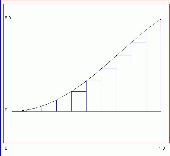
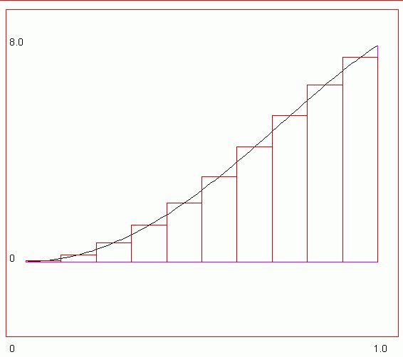
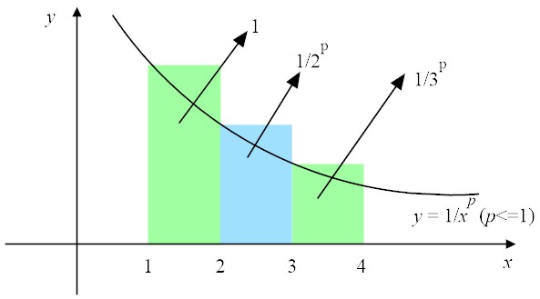
For p < 1, it can be seen from the figure above that

1 +

2^p

3^p

4^p

+ …+

n^p

⌠
⌡

n+1

1

x^p

1 − p

( (1 + n)^1−p − 1 )

→

∞ as n → ∞.

(11)

For p = 1, the above needs to be modified as

1 +

+ …+

⌠
⌡

n+1

1

ln (n + 1)

→

∞ as n → ∞.

(12)

For p > 1,

2^p

3^p

4^p

+ …+

n^p

⌠
⌡

n

1

x^p

p − 1

⎛
⎝

1 −

n^p−1

⎞
⎠

→

p − 1

as n → ∞.

(13)

It is seen that ∑1/n¹⁰ converges faster than ∑1/n³.

Asymptotic notation and Landau-Bachmann magnitude (Big Oh)

The convergence or divergence of an infinite series can be determined by comparing the given series with another series whose convergence/divergence is already known by some other means. The following two definitions can be used to associate the given series with another series.

Definition (Asymptotic notation)

We say that f(x) is asymptotic to g(x) as x → x₀, i.e.

f(x) ∼ g(x) as x → x₀

(14)

when

lim
x→ x₀

f(x)

g(x)

= 1.

(15)

Definition (Bachmann-Landau order of magnitude, aka Big Oh)

We say that f(x) is the Landau order of g(x), i.e.

f(x) = O(g(x)),

(16)

when |f(x)/g(x)| is bounded as x → x₀.

The Big Oh is less restrictive than the asymptotic notation. Note the equal sign (=) used in the Big Oh.

Examples

3 x⁴ + x + 8
x² + 2
∼ 3 x² as x → ∞,
3 x⁴ + x + 8
x² + 2
∼ 4 as x → 0,
3 x⁴ + x + 8
x² + 2
= O(x²) as x → ∞,
3 x⁴ + x + 8
x² + 2
= O(x³) as x → ∞.

Convergence of infinite series

THEOREM (Comparison Test)

Two series, ∑a_n and ∑b_n, of positive terms converge or diverge simultaneously if a_n ∼ b_n as n → ∞.

THEOREM (Comparison Test 2)

If a_n = O (b_n) and ∑b_n converges, ∑a_n converges. The converse is NOT true, i.e. the convergence of b_n is a sufficient condition for the convergence of a_n but not a necessary condition.

Counterexamples

n³

= O(1),

n³

= O(

n³

= O(

n²

) n → ∞.

THEOREM (Ratio Test)

Consider a series ∑a_n of positive terms where |a_n+1/a_n| ∼ r as n → ∞. The series converges if r < 1, diverges if r > 1, no information is gained if r = 1.

Example

The series

∞
∑
n=1

3ⁿ

converges as

⎢
⎢

a_{n + 1}

a_n

⎢
⎢

⎢
⎢
⎢
⎢
⎢

n + 1

3ⁿ⁺¹

3ⁿ

⎢
⎢
⎢
⎢
⎢

⎢
⎢

n + 1

⎢
⎢

→

< 1 as n→ ∞.

THEOREM (Alternating series) Leibniz's test (aka Dirichlet's test)

If a_n > 0 and a_n ↓ 0 (monotonically going to 0) as n → ∞,

S = a₁ − a₂ + a₃ − a₄ + a₅ − a₆ − …,

(17)

converges.

Proof

As S_2n+2 = S_2n+ (a_2n+1−a_2n+2), S₂ < S₄ < S₆ < S₈ …. On the other hand, as S_2n+1= S_2n−1− (a_2n−a_2n+1), it follows S₁ > S₃ > S₅ > S₇ > …. Therefore the interval, [S_2n−1, S_2n], goes to 0 as n→ ∞.

Example

The infinite sum

∞
∑
n=1

(−1)^{n + 1}

= 1 −

−

− …,

converges as a_n = 1/n goes to 0 monotonically.

Note that

∞
∑
n=1

= 1 +

+ …

diverges as this is the p series with p = 1. The latter diverges slowly and the former converges slowly (to ln 2¹).

Exercise of infinite series

∑
⎛
⎝ n² + 2 n −1
n⁴ + 3
⎞
⎠ 3/2

This series is convergent as a_n ∼ 1/n³.
∑
1
(n + 3)^3/2

This series converges as a_n ∼ 1/n^1.5 (p > 1).
∑
n
n² + 3 ln n

This series diverges as a_n ∼ 1/n.
∑
⎛
⎝ 1 + 1
n²
⎞
⎠

This series diverges as a_n ≠ 0 as n → ∞ ².
∑
⎛
⎝ cos n
2 n −1
⎞
⎠ 2

This series converges as

a_n ≤ 1
(2n − 1)²
∼ 1
4 n²
.
∑
(−1)ⁿ ln ⎛
⎝ 1 + 1
√n
⎞
⎠

This series converges per Leibniz's test, i.e ∑(−1)ⁿ is bounded and

ln ⎛
⎝ 1 + 1
√n
⎞
⎠ ↓ 0

as n → ∞.
∑
1
x² + n²

This series converges as a_n = O(1/n²).
∑
(−1)ⁿ
2ⁿ

This series is convergent as |a_n+1/a_n| → 1/2 (ratio test).
∑
ln ⎛
⎝ n² − 1
n² + 1
⎞
⎠

This series converges as

ln ⎛
⎝ n² − 1
n² + 1
⎞
⎠

=

ln ⎛
⎝ 1 − 1
n²
⎞
⎠ − ln ⎛
⎝ 1 + 1
n²
⎞
⎠

∼

− 2
n²
.

Footnotes:

ln (1 + x) = x −

x²

x³

−

x⁴

+ …

Substitute x = 1 to get

ln 2 = 1 −

−

+ …

² Theorem: If ∑a_n converges, a_n → 0 as n → ∞.

(Proof): Assume

∞
∑
i=1

a_i = S.

The partial sum of a_n is defined as

s_n ≡

n
∑
i=1

a_i, a_n = s_n − s_n−1.

As n→ ∞, both s_n and s_n−1 go to S. Hence, a_n → 0.

The equivalent statement to the above is:

If a_n does not go to 0 as n → ∞, ∑a_n diverges.

File translated from T_EX by T_TH, version 4.03.
On 02 Sep 2025, 14:32.