where the coefficients can be determined by substituting
x = a on the both sides and subsequent differentiation as
f(x) = f(a) + f′(a)(x − a) +
f"(a)
2!
(x − a)2 +
f"′(a)
3!
(x − a)3 + …
(2)
Example: Expand f(x) = exp (−1/x2) about x = 0.
One is tempted to use the Taylor series formula, i.e.
f(x) = f(0) + f′(0) x + f"(0)/2! x2 + f"′(0)x3/3! + …. However,
it turns out that all the coefficients are zero as shown in class, i.e.
f(0) = f′(0) = f"(0) = … = 0 so the Taylor series for e−1/x2 is
exp
⎛ ⎝
−
1
x2
⎞ ⎠
= 0 + 0 x + 0
x2
2!
+ …
(3)
This leads us to investigate under what condition the Taylor series is
valid. In fact, this example is a rather pathetic one as
f(z) = e−1/z2 in the complex plane has an essential singularity at
z = 0 as shown in class.
We begin with an identity
⌠ ⌡
x
a
f′(x) dx = f(x) − f(a),
(4)
or
f(x) = f(a) +
⌠ ⌡
x
a
f′(x) dx.
(5)
By replacing f′(x) in Eq.(4) by f"(x), one obtains
is called the remainder of the Taylor series. Note that Eq.(9) is
an identity which holds regardless of the condition of f(x)
(no approximation).
If Rn → 0 as n→ ∞, we say that
f(x) can be expanded by the Taylor series. In the example above
for f(x) = e−1/x2, Rn does not go to 0 as n→ ∞.
The remainder of the Taylor series, Rn, can be assessed if one assumes
that f(n)(x) is bounded as
Note that the convergence range of 1/(1 + x) is |x| < 1 so that the convergence region
of ln x is also |x| < 1.
Rule of 72 (Rule of 70, Rule of 69)
t =
72
r
.
arctan x
By integrating
1
1+x2
= 1 − x2 + x4 − x6 + …,
(19)
one obtains
arctan x = x −
x3
3
+
x5
5
−
x7
7
+….
(20)
Expand ln x about x = 2.
ln x
=
ln ( (x−2)+ 2 )
=
ln
⎛ ⎝
2 (1+
x − 2
2
)
⎞ ⎠
=
ln 2 + ln
⎛ ⎝
1 +
x−2
2
⎞ ⎠
=
ln 2 +
⎛ ⎝
x − 2
2
⎞ ⎠
−
⎛ ⎝
x − 2
2
⎞ ⎠
2
2
+
⎛ ⎝
x − 2
2
⎞ ⎠
3
3
−….
(1 + x)n (binomial expansion)
(1+x)n = 1+ nx +
n (n−1)
2!
x2 +
n (n−1) (n−2)
3!
x3+….
(21)
(Example):
3
√
1003
=
(1000+3)1/3
=
10001/3 (1+0.003)1/3
∼
10
⎛ ⎝
1+0.003 ×
1
3
⎞ ⎠
=
10.01.
Taylor series for multivariable functions
The Taylor series for a single variable function is rewritten as
f(x)
=
f(a) + f′(a) (x−a) +
f"(a)
2!
(x−a)2+
f"′(a)
3!
(x−a)3 +…
=
f(a) +
⎛ ⎝
(x−a)
d
dx
⎞ ⎠
f|a +
1
2!
⎛ ⎝
(x−a)
d
dx
⎞ ⎠
2
f|a +
1
3!
⎛ ⎝
(x−a)
d
dx
⎞ ⎠
3
f|a +…
(22)
When a function, f, has two variables, x and y,
the Taylor series for f(x,y) can be rewritten by replacing
( (x−a)d/dx ) by ( (x−a)∂/∂x +(y−b) ∂/ ∂y) as
f(x,y)
=
f(a,b) +
⎛ ⎝
(x−a)
∂
∂x
+(y−b)
∂
∂y
⎞ ⎠
f|(a,b)
+
1
2!
⎛ ⎝
(x−a)
∂
∂x
+(y−b)
∂
∂y
⎞ ⎠
2
f|(a,b)
+
1
3!
⎛ ⎝
(x−a)
∂
∂x
+(y−b)
∂
∂y
⎞ ⎠
3
f|(a,b)
+
…
(23)
Examples
As noted in class, the formula for the Taylor series can be
bypassed in many cases:
Expand sin (x + y) about (0, 0).
Remembering that sin x = x − x3/3! + x5/5! − …,
sin (x + y) = (x + y) −
(x + y)3
3!
+
(x + y)5
5!
−…
(24)
Expand sin (x + y) about (π, π/2).
In this case, the expansion must contain (x − π)(y − π/2) terms.
sin (x + y)
=
sin
⎛ ⎝
(x − π) +π+ (y −
π
2
)+
π
2
⎞ ⎠
=
sin
⎛ ⎝
(x − π) + (y −
π
2
) +
3π
2
⎞ ⎠
=
sin
⎛ ⎝
(x − π) + (y −
π
2
)
⎞ ⎠
cos
3π
2
+cos
⎛ ⎝
(x − π) +(y −
π
2
)
⎞ ⎠
sin
3π
2
=
(−1) cos
⎛ ⎝
(x − π) + (y −
π
2
)
⎞ ⎠
=
(−1)
⎛ ⎜
⎝
1−
⎛ ⎝
(x − π) + (y −
π
2
)
⎞ ⎠
2
2!
+
⎛ ⎝
(x − π) + (y −
π
2
)
⎞ ⎠
4
4!
− …
⎞ ⎟
⎠
,
where sin (A + B) = sin A cos B + cos A sin B was used.
Expand x2y about (1, 2).
x2y = ( (x−1) + 1)2 ( (y − 2) + 2).
(25)
Expand ln (x + y) about (1, 2).
ln (x + y)
=
ln
⎛ ⎝
(x − 1) + 1 + (y − 2) + 2
⎞ ⎠
=
ln
⎛ ⎝
3 +(x − 1) + (y − 2)
⎞ ⎠
=
ln 3
⎛ ⎝
1 +
(x − 1) + (y − 2)
3
⎞ ⎠
=
ln 3 + ln
⎛ ⎝
1+
(x − 1) + (y − 2)
3
⎞ ⎠
=
ln 3 +
⎛ ⎝
(x − 1) + (y − 2)
3
⎞ ⎠
−
⎛ ⎝
(x − 1) + (y − 2)
3
⎞ ⎠
2
2
+
⎛ ⎝
(x − 1) + (y − 2)
3
⎞ ⎠
3
3
− …
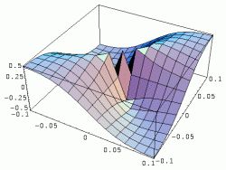
Example of two variable functions
f(x, y) =
⎧ ⎪ ⎨
⎪ ⎩
xy
x2 + y2
(x, y) ≠ (0, 0)
0
(x,y) = (0,0).
(26)
To find out what is lim(x, y)→ (0, 0)f(x,y),
let (x, y) approach to (0, 0) along the line y = x.
By setting x = t and y = t, f(x, y) = t2/(t2 + t2) = 1/2.
However, if one approaches to (0, 0) along the x axis,
f(x, y) = x ×0/(02 + x2) = 0 and they don't match. In short,
f(x, y) does not have the limit as (x, y)→ (0,0).
Chain Differentiation
When f(x, y) is a composite function (i.e. x and y are also functions
of other variables), the derivative of f with respect to the implicit variable
can be achieved by using the chain differentiation rule, i.e.
df
dt
=
∂f
∂x
dx
dt
+
∂f
∂y
dy
dt
.
(27)
An example was shown in class, i.e. this is a variation of
derivative of composite functions.
Footnotes:
1
If one substitutes x=1 on the both sides, one obtains
ln 2 = 1 −
1
2
+
1
3
−
1
4
+
1
5
− …
(28)
Note that
1 +
1
2
+
1
3
+
1
4
+
1
5
+ …,
(29)
diverges.
File translated from
TEX
by
TTH,
version 4.03. On 24 Aug 2025, 16:53.