


| (1) |
| (2) |
| (3) |
|
| (4) |
|
| (6) |
 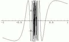 |
 Note that f(x) is sandwiched from both sides as
| (7) |
| (8) |
| (9) |
|
| (11) |
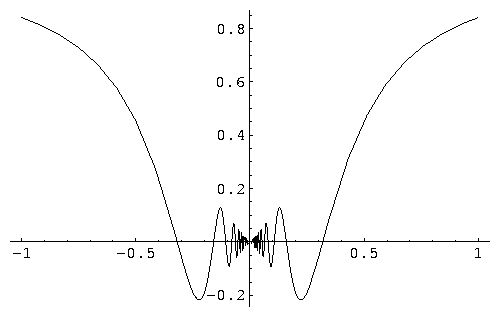
 Note that in this case, f(x) behaves much gently around x=0 because
x2 (the magnitude of f(x)) approaches to 0 more quickly than x.
The function, f(x), is continuous at x = 0 using the same logic as in the previous example.
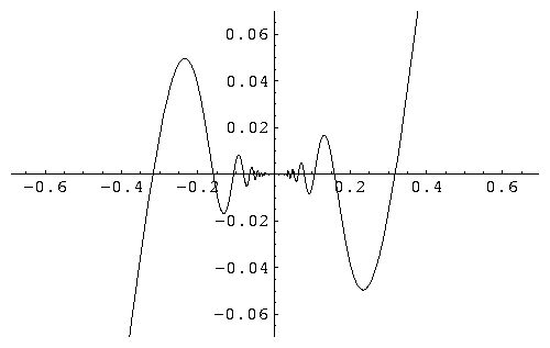
For differentiability,
Note that in this case, f(x) behaves much gently around x=0 because
x2 (the magnitude of f(x)) approaches to 0 more quickly than x.
The function, f(x), is continuous at x = 0 using the same logic as in the previous example.
For differentiability,
|
| (13) |
|
|
|
|
| x | f(x) |
| 1 | 1 |
| 2 | 8 |
| 3 | 27 |
| 4 | 64 |
| 5 | 125 |
| 6 | 216 |
 It is possible to numerically differentiate a given function
using all available data points.
What is known from the table is the difference of f(x), i.e.
It is possible to numerically differentiate a given function
using all available data points.
What is known from the table is the difference of f(x), i.e.
| (14) |
| (15) |
|
| (17) |
| (18) |
| (19) |
| (20) |
| (21) |
| (22) |
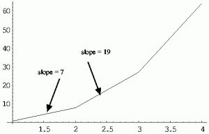
| x | f(x) | ∆f | ∆2 f | ∆3 f | ∆4 f |
| 1 | 1 | 7 | 12 | 6 | 0 |
| 2 | 8 | 19 | 18 | 6 | X |
| 3 | 27 | 37 | 24 | X | X |
| 4 | 64 | 61 | X | X | X |
| 5 | 125 | X | X |
|