Write C programs for the following:
1.
Solve the following 10 simultaneous equations by the Gauss-Jordan elimination method.
|
| ⎧
⎪
⎪
⎪
⎨
⎪
⎪
⎪
⎩
|
|
a11 x1 + a12 x2 + a13 x3 + …+ a1 10x10 = c1 |
|
|
a21 x1 + a22 x2 + a23 x3 + …+ a2 10x10 = c2 |
|
|
a31 x1 + a32 x2 + a33 x3 + …+ a3 10x10 = c3 |
|
|
|
an1 x1 + an2 x2 + an3 x3 + …+ a10 10x10 = c10 |
|
|
|
| (1) |
where aij is given as
a[10][10]={
{3.55618, 5.87317, 7.84934, 5.6951, 3.84642, 9.15038, -1.68539, 5.03067, 7.63384, -1.75626},
{-4.82893, 8.38177, -0.301221, 5.10182, -4.1169,-6.09145, -3.95675, -2.33365, 1.3969, 6.54555},
{-7.64196, 5.66605,3.20481, 1.55619, -1.19814, 9.79288, 5.35547, 5.86109, 4.95544, -9.35749},
{-2.95914, -9.16958,7.3216, 2.39876, -8.1302, -7.55135, -2.37718, 7.29694, 5.9867, 8.5401},
{-8.42043, -0.369407, -5.4102, -8.00545, 9.22153, 3.96454, 5.38499, 0.438365, 0.419677, 4.17166},
{6.02952, 4.57728, 5.46424, 3.52915, -1.01135, -3.74686,8.14264, -8.86961, -2.88114, 1.29821},
{0.519819, -6.16655, 1.13216, 2.75811, -1.05975, 4.20286, -3.45764, 0.763558, -0.281287, -9.76168},
{5.15737, -9.67481, 9.29904, -3.93334, 9.12785, -4.25208, -6.1652, 2.5375, 0.139195, 2.00106},
{-4.30784, 1.40711, -6.97966, -9.29715, 5.17234, 2.42634, 1.88818, -2.05526, -3.7679, 3.3708},
{-4.65418, 7.18118, 6.51338, 3.13249, 0.188456,  -16.85599, 7.21435, -2.93417, 1.06061, 1.10807}
};
and ci is given as
c[10]={-1.92193, -2.35262, 2.27709, -2.67493, 1.84756, 4.154126, -0.93387, -1.28356, -3.46841, -2.61529};
2.
Solve the following set of nonlinear equations by the Gauss-Seidel method.
Start with an initial guess of x = y = z = 1.
3.
(a) Derive the formula similar to Equation (17) in the
07/21 lecture note
but at x = b (last point).
(b)
The altitude (ft)
from the sea level and the corresponding time (sec) for a fictitious rocket were measured as follows:
| Time | 0 | 20 | 40 | 60 | 80 | 100 | 120 | 140 | 160 | 180 | 200 |
| Altitude | 370 | 9170 | 23835 | 45624 | 62065 | 87368 | 97355 | 103422 | 127892 | 149626 | 160095 |
Numerically compute the velocity from the table above for t = 0 ∼ 200 keeping the same accuracy as the central difference scheme.
At t=0, use Equation (17) in the
07/21 lecture note and
at t=200, use the formula you derived in (a).
4.
(a) Evaluate analytically
(b) Write a C program to numerically integrate the above using the Simpson rule.
Note that the graph of x ln x looks like
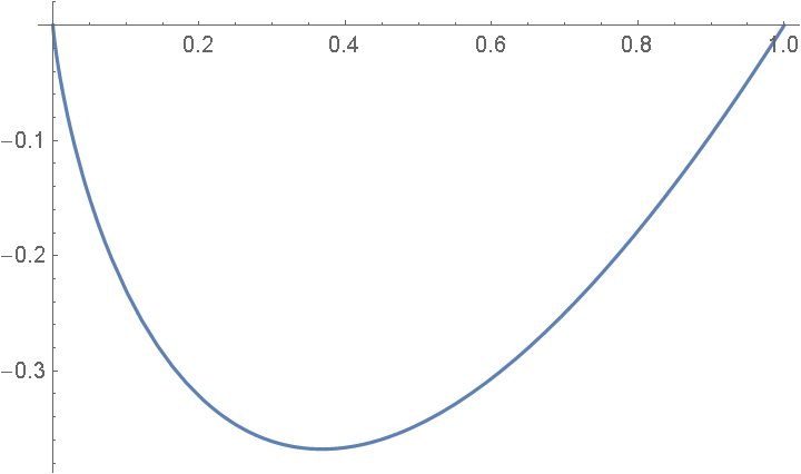 Note also that ln x → − ∞ as x → 0. So the challenge is how to handle the seemingly singular point of x = 0.


