#include <stdio.h>
#include <math.h>

#define N 10

int main()
{
  float x[]={ -4.0, 1.2, 1.3, 2.5, -12.7,
   9.0, 1.41, 65.2, -2.1, 2.36};
  int i;
  float sum = 0.0, average, variance;

  for (i=0; i<N; i++) sum+=x[i];
  average=sum/N;

  for (i=0; i<N; i++)
   variance += pow(x[i]-average, 2);
  variance = variance/(N-1);

  printf("avg.= %f std. dev. = %f \n ",
    average, sqrt(variance));
  return 0;
}
|
|
      PARAMETER(N=10)
      REAL X(N), SUM, AVE, VAR
      INTEGER I

      DATA X /-4.0,1.2,1.3,2.5,-12.7,9.0,1.41,
     c 65.2,-2.1, 2.36/

      SUM=0.0

      DO 10 I=1,N
       SUM=SUM+X(I)
 10   CONTINUE

      AVE=SUM/FLOAT(N)

      DO 20 I=1,N
       VAR=VAR+(X(I)-AVE)**2
 20   CONTINUE
      VAR=VAR/(FLOAT(N)-1.0)

      WRITE(*,*) "Average=", AVE,
     c  ' Standard deviation =', SQRT(VAR)
      STOP
      END
|
|


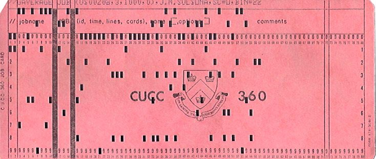
 FORTRAN (FOrmulaTRANslation) was created a half century ago and was the de-facto
programming language for engineers and scientists until recently because of the
inertia and a vast amount of subroutines written (and fully debugged).
Although it's rare these days that you write a large program in FORTRAN from scratch,
it is still important that you are able to read a FORTRAN program somebody wrote before.
FORTRAN (FOrmulaTRANslation) was created a half century ago and was the de-facto
programming language for engineers and scientists until recently because of the
inertia and a vast amount of subroutines written (and fully debugged).
Although it's rare these days that you write a large program in FORTRAN from scratch,
it is still important that you are able to read a FORTRAN program somebody wrote before.