


clc % clears screen 1+3 2^12 (3+2*i)*(2-4*i) % complex algebra abs(4-3*i) %absolute value sin(pi) cos(2*pi) log(2.718) %natural logarithm log2(1024) log10(1000) format long sqrt(5) pi format short sqrt(3) |
a=20.0 b=a-sin(3); a+b clear a a |
i %imaginary number j % same as i clock % current time (six elements) date % current date pi %3.14156 eps %smallest tolerance number in the system format long pi pi=2.14 pi clear pi pi |
v1=[1 2 3] % defines a 3-D row vector. v1=[1, 2, 3] % Same as above. Separator is either space or comma v2=[1;2;3] % this defines a column vector. v2=v1' %transpose of v1, i.e. column vector m1=[1 2 3;4 5 6;7 8 9] %defines a 3x3 matrix m1=[1,2,3;4,5,6;7,8,9]; %semicolon suppresses echo m2=[-4 5 6; 1 2 -87; 12 -43 12]; m2(:, 1) % Extracts the first column m2(2, :) % Extracts the second row m2(2,3)=10; % Assigns 10 to the (2,3) element of m2. m1*v2 %matrix multiplication inv(m1) %inverse of m1 [vec, lambda] = eig(m1) % eigenvectors and eigenvalues of m1 m1\m2 % inverse of m1 times m2, same as inv(m1)*m2 m1*v2 % matrix m1 times vector v2 a=eye(3) % 3x3 identity matrix a=zeros(3) % 3x3 matrix with 0 as components a=ones(3) % 3x3 matrix with 1 as components det(m1) % determinant of m1 |
|
 a=[1 4 5; 8 1 2; 6 9 -8];
 b=[4; 7; 0];
 sol2 = inv(a)*b
   % or
 sol2 = a\b
x=[1: 2 :10]; % a sequence between 1 and 10 with an increment of 2. x=linspace(1, 9, 5); a sequence between 1 and 9 with equidistant 5 entries y=x; z=x * y % error z = x .* y; %works z = x / y ; %error z = x ./y ; % works |
x=[0:0.1:10]; %initial value, increment, final value
y=sin(x);
plot(x, sin(x)); %calls Gnuplot


x=linspace(0,2, 20) % between 0 and 2 with 20 divisions
plot(x, sin(x))
%%%%%%%%%%%%%%%%%%
x=[0: 0.2 : 10];
y=1/2 * sin(2*x) ./ x;
xlabel('X-axis');
ylabel('sin(2x)/x');
plot(x, y);

close;
%%%%%%%%%%%%%%%%%
t=[0: 0.02: 2*pi];
plot(cos(3*t), sin(2*t))

%%%%%%%%%%%%%%%%%%%%
x=[0: 0.01: 2*pi];
y1=sin(x);
y2=sin(2*x);
y3=sin(3*x);
plot(x, y1, x, y2,x, y3);
%%%%%%%%%%%%%%
xx=[-10:0.4:10];
yy=xx;
[x,y]=meshgrid(xx,yy);
z=(x .^2+y.^2).*sin(y)./y;
mesh(x,y,z)
surfc(x,y,z)
contour(x,y,z)
close
|
MATLAB generated graph
a=[1 2 3 4 5] % defines x4+2x3+3x2+4x+5 r=roots(a) % solves x4+2x3+3x2+4x+5=0. |
disp(a)
disp('Enter a number = ')
a=input('Enter a number =');
fprintf('The solution is %f\n', a);# %f and %d are available but not %lf
|
cd c:\tmp cd 'c:\users\sn\documents' pwd % present working directory cd % back to home directory myownfile % loading a script m-file named "myownfile.m" save myown.txt a, b % saves variables "a" and "b" to a file "myown.txt" load myown.txt |
function y=myfunction(x) y=x^3-x+1; end |
function [x, y]=myfunction2(z) x=z^2; y=z^3; end |
[a,b]=myfunction2(3); |
if a>2
 disp('a is larger than 2')
end

for k=0:2:10
 disp(2*k)
end
|
|
|
|
|
|
|
|
|
|
|
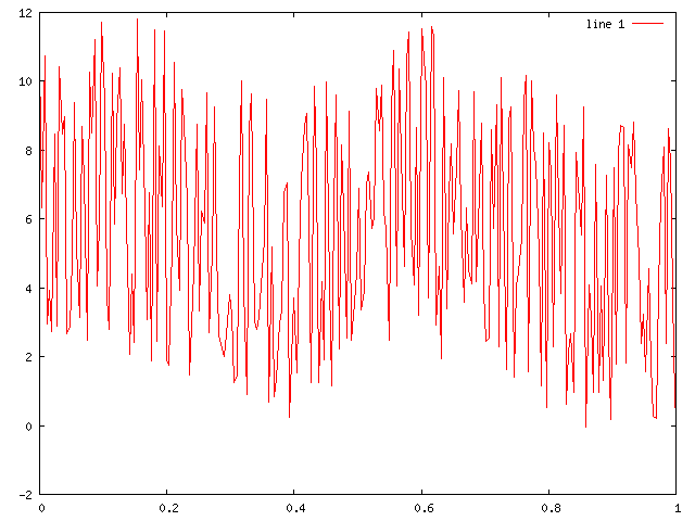 Using the fft (Fast Fourier Transform) and ifft
(Inverse Fourier Transform)
functions in MATLAB/OCTAVE, remove the noise from the data above and restore the original signal.
To import the data for the graph above into Octave/MATLAB, copy the following line and paste it into an Octave/MATLAB window.
Using the fft (Fast Fourier Transform) and ifft
(Inverse Fourier Transform)
functions in MATLAB/OCTAVE, remove the noise from the data above and restore the original signal.
To import the data for the graph above into Octave/MATLAB, copy the following line and paste it into an Octave/MATLAB window.
y=[10.5998892219547 6.32715963943755 10.7418564397819 2.9411380441864 3.92528722303704 2.71618105372149 8.4617982675031 2.88080944171953 10.4141369874892 8.476032583145489 8.964925641878001 2.67576180217924 2.85081602904105 4.85231952204638 9.38358373297042 5.16481823892903 3.14070937711815 8.699875412947099 7.21927535505636 2.47218681863012 10.2726165797325 8.500254531789301 11.1978723384108 4.05021576256659 5.77322285188005 11.7074336020358 9.400871264109419 3.71878673302725 2.78562995675663 10.2401630961987 5.84306139392084 8.82789975382806 10.3993315932854 6.74306607935596 8.750462753122729 5.90480261238712 2.06109189130585 4.40535088299872 2.41192556568313 11.8214297012451 7.44250415683415 10.032769833142 6.28901765997294 3.08186615850219 6.76595055198963 1.87944040723309 11.502034897292 2.44379054233261 8.128891862212489 6.34299932572315 11.4665531337537 1.86621678597553 1.75517155481136 5.19324241215718 10.5420445171336 5.82311606131353 3.92802666444074 9.77260830545065 8.76106471812958 6.54554696769744 1.4624210554122 2.92068844004011 4.48263396519447 8.739554957492571 3.33478186865148 6.24348148116228 5.87860301757644 9.666406406463951 2.70299316464037 5.01601721808914 9.26536386544738 5.09532896085959 2.62513156468079 2.21732831519875 1.99448077033047 2.62844514632015 3.79686487481322 3.24327464459272 1.2326443145944 1.45988948327978 7.1131310391548 10.0220774080567 3.93470053413877 0.894329071535874 8.60989560717546 9.63540704314247 3.00857673282652 2.79007156060591 3.15054286446995 4.53048193808516 5.38399703002467 9.4833604924008 0.6953758598942 5.19383112351193 0.844822890049153 1.34649332130299 2.98525367766063 3.31627989414972 6.76285368200212 7.04875327912278 0.251045988826941 1.9108517787023 3.69941930619919 1.52517099472442 4.831074892421 7.11794613059188 8.72763093617244 9.078887558695371 5.89633680306463 1.24117091269616 9.850706571849731 7.44945101897683 1.24091019808261 4.18876971107157 1.9176033724533 9.995859008983791 4.06138975672046 1.15781821760705 6.39682907701427 9.58794591991612 2.2193562129817 8.15089615664534 6.25502635127747 2.54857914360014 9.129606203212679 2.4736245862179 3.56168512084511 4.43958848222138 6.8931750450365 3.37222234736257 3.90894160047792 7.00239599243425 7.36043668237722 5.72237545873726 6.02879296664729 9.802065832144031 8.575987244312429 9.897577054258401 6.18523789886617 5.69121169822893 2.46963366954875 9.129229771930889 10.8952016844065 4.04009660589757 10.3743854729916 7.86000365182057 4.62415698798384 10.6214785584302 11.4224951621026 5.67326994393055 4.08637580957679 8.65738342494789 3.19239876321067 11.5201022637337 10.636312915602 9.82811239395342 3.70890071720701 11.5798531399931 11.3079723127561 2.91023922097878 4.62563348751362 1.94134261430337 10.1199743509774 3.39739911000981 6.74500334449411 8.170425024996179 5.56015657871609 7.5183998639944 9.724435694474771 6.0923080693899 3.59482558370596 6.31863247939307 4.52463371931999 4.10296747447814 9.695171467636451 4.18461466022538 5.80815539286633 8.77375948273572 3.89726672007424 2.4379111867341 2.53028144217005 8.599734675735849 5.73721564890586 9.31292716873403 2.30164223598104 10.1205267404267 6.46257375724972 1.61357790565941 8.83703123702375 9.241195975932539 1.39848359552096 4.04514624784499 4.45713558113789 5.40256645503303 9.458465543021051 10.1594053991668 1.57320417124056 10.025068241083 8.050843440082611 7.57425636264847 4.99279654689739 1.14890755632154 8.48815583223322 0.513616604704808 8.20951495224771 7.36944262027792 2.28314474381409 9.61805543347821 6.38395393390104 3.82496380452266 8.716233740636451 0.624777553892277 2.13639412542771 2.67182229714328 0.960693039360867 7.94782117163402 6.97092617961824 5.54658352916538 9.25358919832107 -0.0518943288602689 4.09372366108078 3.0771241498034 0.9687056105548451 7.58002335011327 0.964153518012499 4.05886921736417 1.30771587473559 7.28546269899251 2.60725514587506 0.181148813423656 7.50124107556926 1.78225486901118 7.93044999804643 8.726414919885549 8.64856640820909 1.81661636398602 8.15011697120986 7.48520651711012 8.821324599765621 6.77111885101838 4.83400122253399 2.39038025124365 3.22625506903038 1.55735245264944 4.56184163155081 1.75825250678772 0.269608991651202 0.197345665382678 4.06499325144136 6.52779016528276 8.09415174197148 2.37792649587988 8.6329654872403 7.66695265328003 1.99742029842287 0.0182366166899817];To change the working directory, issue
cd c:/tmp |
cd c:/tmp % CD to the "c:/tmp" directory % plot(y); f1=fft(y); % Fast Fourier Transform of y, i.e. frequency domain expression of y plot(abs(f1)); % Since f1 is a set of complex numbers, we take only the absolute values. % % Examine the graph of f1 (in frequency) and determine the cut-off values. % % Passing only low frequency data (low pass filter) % for i=1:256 if abs(f1(i)) < (your guess) f1(i)=0; end; end; % % Inverse FFT on f1 % y2=ifft(f1); % % y2 is real but there is some dust so chop them off. % y2=abs(y2); plot(y2); |